Structured ModeL reductIon (SiMpLIfy) Toolbox for MATLAB

User's Guide for Structured ModeL reductIon (SiMpLIfy) Toolbox

Authors:
Martin Biel, Farhad Farokhi, Henrik Sandberg

Download:
The MATLAB codes for the toolbox can be downloaded from [toolbox (August 15, 2014)]. The PDF version of this user guide can be downloaded from [manual (August 15, 2014)]. Please kindly see Installation for more information on installing the toolbox.

We have created a permanent webpage for the toolbox on http://simplifytoolbox.tumblr.com/

Communication:
For comments, bug reports, encouragement, suggestions, and complaints, please send email to farokhi@ee.kth.se

If you use SiMpLIfy for research purposes, we would be happy to hear about it and mention it in the reference guide, please send email to farokhi@ee.kth.se

Citation:
M. Biel, F. Farokhi, H. Sandberg, “Structured ModeL reductIon (SiMpLIfy) Toolbox for MATLAB,” Technical Report, KTH Royal Institute of Technology, Stockholm, Sweden, 2014.

1 Introduction
1.1 Overview of interconnected linear systems
1.2 About the toolbox
1.3 Key features
1.4 Installation
1.5 Requirements
2 Getting started
2.1 Creating an interconnected linear systems
2.2 Using the ‘SystemNetwork’ class features
2.3 Generating a Simulink model
3 Model reduction of an interconnected linear system
3.1 Analysing the system
3.2 Reducing the order of the system
3.3 Improving the model reduction
A Examples
A.1 Frequency weighted balanced reduction
A.2 A mechanical example
B ‘SystemNetwork’ Class Reference
B.1 Properties
B.2 Class constructor
B.3 Methods
  B.3.1 changeSubsystems
  B.3.2 extractSubsystems
  B.3.3 getStateSizes
  B.3.4 computeGramians
  B.3.5 computeGeneralisedGramians
  B.3.6 extractSubgramians
  B.3.7 structuredTransformation
  B.3.8 singularPerturbation
  B.3.9 createParametricStructuredRealisation
  B.3.10 generateSimulinkModel
C Function Reference
C.1 balancedNetworkReduction
C.2 compareHankels
C.3 computeStructuredHankels
C.4 improveNetworkReduction

1 Introduction

1.1 Overview of interconnected linear systems

An Interconnected linear system is a collection of linear systems that are connected in some network structure. In an interconnected system, the subsystems are stored in a block diagonal structure $$ G(s) = \begin{pmatrix} G_1(s) & & 0 \\ & \ddots & \\ 0 & & G_n(s) \end{pmatrix} := \left(\begin{array}{c|c} A_G & B_G \\ \hline C_G & D_G \end{array}\right) $$

where $n$ is the total number of subsystems. The state space matrices $A_{G}, B_{G}, C_{G}$ and $D_{G}$ are block diagonal matrices consisting of the state space matrices of the subsystems. The network that describes the interconnections between the subsystems is stored as

N = (\begin{matrix} D_{E} & D_{F} \\ D_{H} & D_{K} \end{matrix})

where the $D$ components are adjacency matrices for the internal connections, external inputs and outputs and external connections. Note that the data representation used only supports scalar connections and does not include any dynamics present in the network. However, if the network contains dynamics, then they can be included in the subsystems during calculations.

The complete dynamics of the interconnected system can be attained through the structured realisation, defined as $$ F(N,G) := \left(\begin{array}{c|c} A_G+B_GMD_KC_G & B_GMD_H \\ \hline D_FLC_G & D_E+D_FD_GMD_H \end{array}\right) := \left(\begin{array}{c|c} A & B \\ \hline C & D \end{array}\right) $$

where

L : = {(I - D_{G} D_{K})}^{- 1}, M : = {(I - D_{K} D_{G})}^{- 1}

A more detailed definition and analysis of interconnected linear systems can be read in [2].

1.2 About the toolbox

The Interconnected linear systems toolbox contains various functions and a data structure for working with interconnected linear systems. The main usage of the toolbox is structure preserving model reduction of interconnected systems, but there are other features as well. The model reduction techniques and the representation of the interconnected systems are based on [2].

1.3 Key features

Data representation of an interconnected linear system
Structure preserving model reduction
Simulink-model generation

1.4 Installation

Copy the directory “sysnettools” into Matlab’s toolbox folder and add the path to the MATLAB search path. See path, in the MATLAB documentation for more information.

1.5 Requirements

The toolbox was written in Matlab version 8.1 (R2013a) and requires the Control toolbox and the Robust Control toolbox. Also, the method ‘computeGeneralisedGramians’ (B.3.5) requires the CVX software, available at CVX Research.

2 Getting started

2.1 Creating an interconnected linear systems

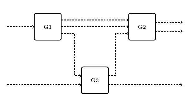
Consider the interconnected linear system that consists of the following subsystems:

G_{1} = (\begin{matrix} \frac{1}{s + 1} \\ \frac{1}{{(s + 3)}^{2}} \\ \frac{s}{s + 1} \end{matrix}), G_{2} = (\begin{matrix} \frac{s + 1}{s + 3} & \frac{1}{(s + 1) (s + 2)} & \frac{1}{2 s + 5} \\ 0 & \frac{1}{s + 1} & \frac{1}{s + 1} \end{matrix}), G_{3} = (\begin{matrix} \frac{1}{s + 2} & 0 \\ 0 & \frac{1}{s + 3} \end{matrix})

connected according to the structure shown in Fig.1

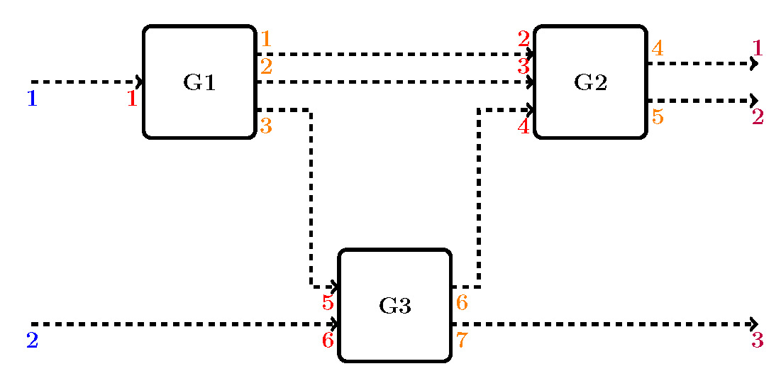
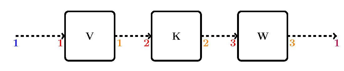
Figure 1: Network structure of an interconnected linear system.

To construct an instance of ‘SystemNetwork’ that describes this structure, label the inputs and outputs as has been done in Fig.2. Start with the first subsystem G1, label its inputs (shown in red) in consecutive order, then keep labelling the inputs of the remaining subsystems following the same order. The same procedure is repeated for the outputs (shown in orange) of the subsystems. Also, the external inputs and outputs (shown in blue and purple respectively) need to be labelled in the same way. The edges of the network can now be described by 4 arrays. The first describes the internal connections:

i n t e r n a l E d g e s = (\begin{matrix} 1 & 2 \\ 2 & 3 \\ 3 & 5 \\ 6 & 4 \end{matrix})

Here, the first row $(1, 2)$ means that there is a connection between output 1 (which belongs to G1) to input 2 (which belongs to G2). Likewise, the external connections are described by:

e x t e r n a l I n p u t E d g e s = (\begin{matrix} 1 & 1 \\ 2 & 6 \end{matrix}), e x t e r n a l O u t p u t E d g e s = (\begin{matrix} 4 & 1 \\ 5 & 2 \\ 7 & 3 \end{matrix})

Check that these edge-lists match the connections in Fig.2. Finally, if there are any connections between the external inputs and outputs they should be described in the array ‘externalEdges’. However, in this case, there are no such connections and an empty list is supplied instead.

Figure 2: Network structure where all internal and external inputs and outputs have been labelled in consecutive order.

An instance of the ‘SystemNetwork’ class can now be created using the following code:

s = tf(’s’);
g1 = ([1/(s+1) ; 1/(s+3)^2 ; s/(s+1)]);
g2 = ([(s+1)/(s+3) 1/((s+1)*(s+2)) 1/(2*s+5) ; 0 1/(s+1) 1/(s+1)]);
g3 = ([1/(s+2) 0 ; 0 1/(s+3)]);

iedges = [1 2 ; 2 3 ; 3 5 ; 6 4];
einedges = [1 1 ; 2 6];
eoutedges = [4 1 ; 5 2 ; 7 3];
eedges = [];

systemNetwork = SystemNetwork(iedges,einedges,eoutedges,eedges,g1,g2,g3)

It is important that the subsystems are entered in the same order as they were labelled.

2.2 Using the ‘SystemNetwork’ class features

Check the current properties of the class that was just created

>> systemNetwork
 

 
systemNetwork =
 

 
  SystemNetwork with properties:
 

 
            numberOfNodes: 3
 
               subsystems: [7x6 ss]
 
    structuredRealisation: [3x2 ss]
 
           controlGramian: []
 
           observeGramian: []
 
              gramianType: ’uncalculated’
 
                  network: [1x1 struct]

The ‘subsystems’ property contains the subsystems in the form of (1.1), ‘network’ contains the network structure in the form of (1.1) and ‘structuredRealisation’ contains the structured realisation as in (1.1). Also, one can observe that there are $3$ subsystems in this structure and that the Gramians have not been yet calculated. To calculate Gramians, use for example the ‘computeGramians’ (B.3.4) method:

>> systemNetwork = systemNetwork.computeGramians

systemNetwork =

  SystemNetwork with properties:

            numberOfNodes: 3
               subsystems: [7x6 ss]
    structuredRealisation: [3x2 ss]
           controlGramian: [11x11 double]
           observeGramian: [11x11 double]
              gramianType: ’regular’
                  network: [1x1 struct]

One can now observe that ‘regular’ Gramians, which are the controllability and observability Gramians of the structured realisation, have been calculated. These can be observed in the properties ‘controlGramian’ and ‘observeGramian’.

To analyse the individual subsystems in the structure, use the method ‘extractSubsystem’ (B.3.2), which returns the state space of the desired subsystem. For example:

>> tf(systemNetwork.extractSubsystem(1))

ans =

  From input to output...
         1
   1:  -----
       s + 1

             1
   2:  -------------
       s^2 + 6 s + 9

         s
   3:  -----
       s + 1

Continuous-time transfer function.

which can be recognized as

G_{1}

specified in (2.1). Also, one can extract the part of the controllability Gramian that originates from subsystem

G_{1}

using the method ‘extractSubgramians’ (B.3.6) as:

>> [p,q] = systemNetwork.extractSubgramians(1);
 
>> p
 

 
p =
 

 
    0.5000    0.0312    0.1250    0.5000
 
    0.0312    0.0208    0.0000    0.0312
 
    0.1250    0.0000    0.0370    0.1250
 
    0.5000    0.0312    0.1250    0.5000

The method assumes that Gramians have been calculated using either of the methods ‘computeGramians’ (B.3.4) or ‘computeGeneralisedGramians’ (B.3.5).

2.3 Generating a Simulink model

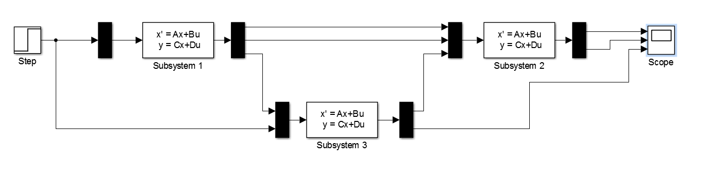
The recently created instance of ‘SystemNetwork’ can be used to generate a Simulink model of the interconnected system. The method ‘generateSimulinkModel’ (B.3.10) returns a handle to the simulation:

>> systemNetwork.generateSimulinkModel(’sysnetExample’)

and also opens a Simulink window, shown in Fig.3, displaying the simulation.

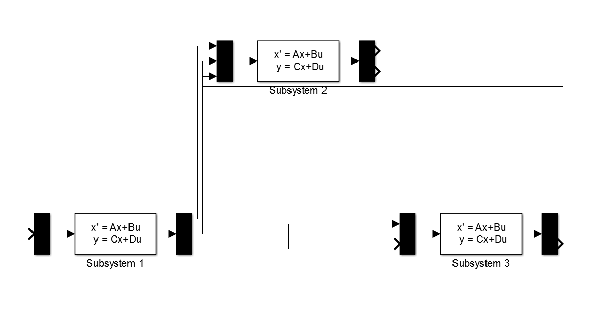
Figure 3: Generated simulink model of an interconnected linear system.

Note that the external inputs and outputs of the interconnected system have not been connected and desired sources and sinks have to be added manually. It is not possible to automatically connect the ports in a neat way, so to enhance readability they have to be arranged manually. For example, the model that was just generated can be arranged to resemble the structure in Fig.1. A manual arrangement with an added step input and sink is shown in Fig.4. The generated simulation can be used to observe the network structure and analyse the dynamics of the system.

Figure 4: Generated Simulink model with arranged port connections and added source and sink.

An interconnected system with a great number of subsystems and internal connections may not be generated in a readable way and can be troublesome to arrange manually.

3 Model reduction of an interconnected linear system

The aim is to reduce the overall order of an interconnected linear system, while preserving the internal structure and capturing the total input-output behaviour of the original system as well as possible. The model reduction techniques suggested in [2] are implemented in the toolbox and will be used to reduce the system created in section 2.1.

3.1 Analysing the system

Begin with an analysis of the system similar to when regular balanced order reduction is performed. Use the method

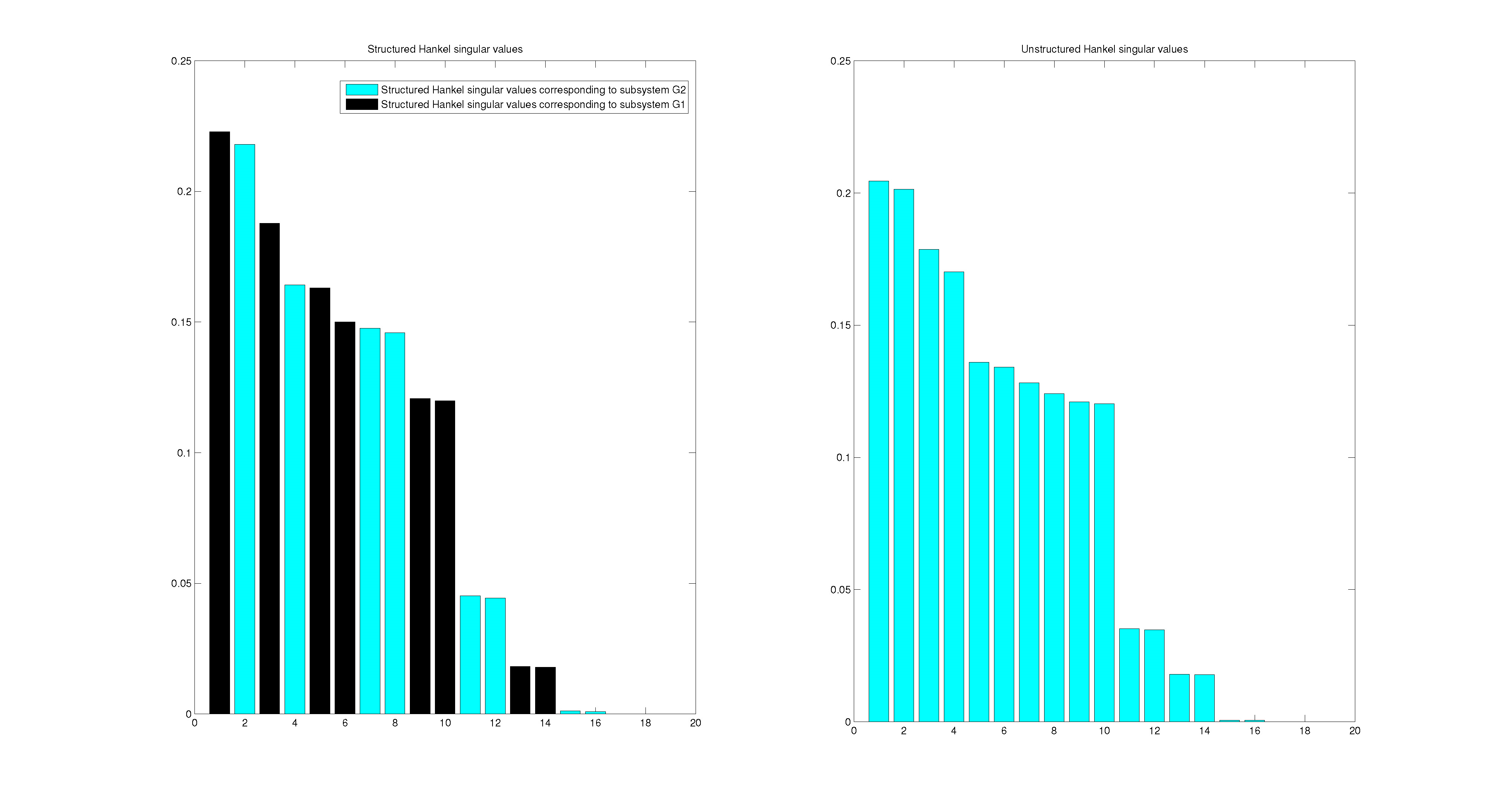
>> compareHankels(systemNetwork)

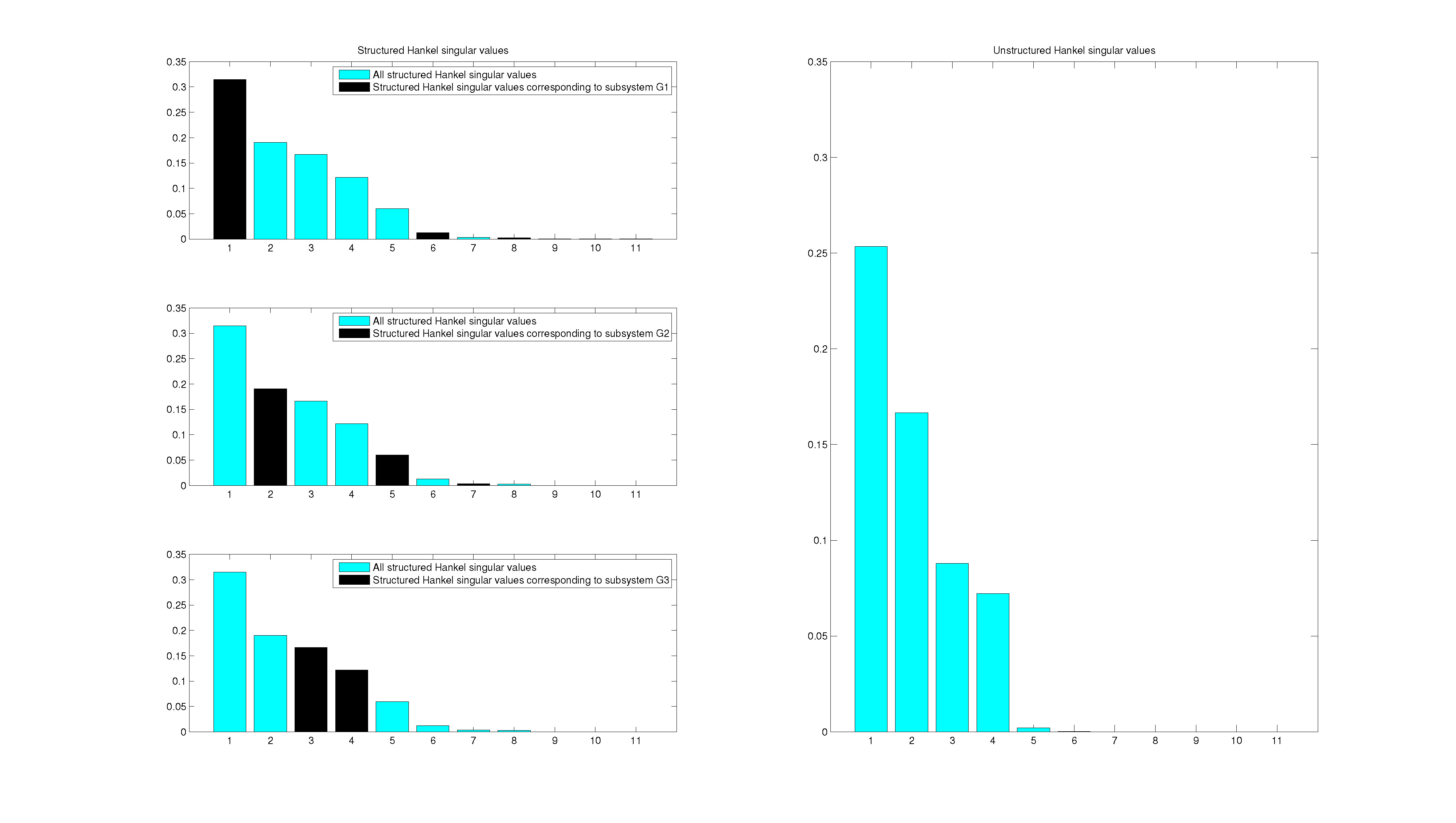
Figure 5: Structured and unstructured Hankel singular values of an interconnected linear system.

If the interconnected system is treated as one system, with no regard to the internal structure, the rightmost part of Fig.5 is acquired. The plot shows the Hankel singular values of the entire system and the relative sizes indicate that $4$ states is enough to capture the dynamic behaviour. The total system would then be reduced by for example balanced truncation, keeping only $4$ states. This method might yield a good approximation of the interconnected systems’ overall behaviour, but the internal structure is lost.

When structure is taken into consideration, the left part of Fig.5 is acquired. The plot shows the structured Hankel singular values, defined in [2], and also highlights which values comes from which system. Applying the same heuristics, the plot suggests that $5$ states are required to achieve a good approximation. In this case, the prize for preserving the internal structure appears to be to keep one more state when reducing the order.

Looking at the relative sizes of the Hankel values in the individual subsystems suggests the following order reduction scheme:

subsystem 1: Keep $1$ state
subsystem 2: Keep $2$ states
subsystem 3: Keep $2$ states

The interconnected linear system can now be reduced.

3.2 Reducing the order of the system

Perform the model reduction of the interconnected system suggested in the previous section by

                                                                                  
                                                                                  
>> red = balancedNetworkReduction(systemNetwork,[1 2 2])
 

 
red =
 

 
  SystemNetwork with properties:
 

 
            numberOfNodes: 3
 
               subsystems: [7x6 ss]
 
    structuredRealisation: [3x2 ss]
 
           controlGramian: [5x5 double]
 
           observeGramian: [5x5 double]
 
              gramianType: ’regular’
 
                  network: [1x1 struct]

Note that supplying an empty list instead of the deduced sizes will show the plots of the structured Hankel singular values in Fig.5 separately in series and prompt for the size each subsystem shall be reduced to.

As an indication on how well the reduced system approximates the original system, observe the system gains shown in Fig.6.

Figure 6: Largest and smallest singular values of the original and the reduced interconnected systems.

The difference in $H_{\infty}$ norm is given by

>> norm(systemNetwork.structuredRealisation-red.structuredRealisation,inf)
 

 
ans =
 

 
    0.0114

The function defaults to performing a balanced truncation. Instead, singular perturbation of each subsystem can be used by supplying options to the method. When using such an approach, the reduced system will exactly match the original system at zero frequency instead of infinite frequency. Reduce the interconnected system using singular perturbation by

>> red = balancedNetworkReduction(systemNetwork,[1 2 2],’ReductionMethod’,’perturbation’)

The difference in

H_{\infty}

norm is now given by

>> norm(systemNetwork.structuredRealisation-red.structuredRealisation,inf)
 

 
ans =
 

 
    0.0174

which in this case is not an improvement.

Also, one can try to use block structured Gramians using instead

                                                                                  
                                                                                  
>> red = balancedNetworkReduction(systemNetwork,[1 2 2],’GramianType’,’generalised’)

The use of such Gramians, if they exist, and their benefits is further discussed in [2].

3.3 Improving the model reduction

The reduction performed in the previous section can be improved through numerical optimization techniques. The function ‘improveNetworkReduction’ makes use of the ‘hinfstruct’ method, based on [1], from the “Robust control toolbox”. Improve the model reduction by

>> optred = improveNetworkReduction(systemNetwork,red)
 
Start: Peak gain = 0.011414
 
Final: Peak gain = 0.000129, Iterations = 300
 

 
optred =
 

 
  SystemNetwork with properties:
 

 
            numberOfNodes: 3
 
               subsystems: [7x6 ss]
 
    structuredRealisation: [3x2 ss]
 
           controlGramian: []
 
           observeGramian: []
 
              gramianType: ’uncalculated’
 
                  network: [1x1 struct]

where “red” is the reduced system acquired through balanced truncation in the previous section. Notice that there is a remarkable decrease in

H_{\infty}

norm and the reduced system can be said to approximate the original system better than before.

References

[1] P. Apkarian and D. Noll. Nonsmooth h infin; synthesis. Automatic Control, IEEE Transactions on, 51(1):71–86, Jan 2006.

[2] Henrik Sandberg and Richard M Murray. Model reduction of interconnected linear systems. Optimal Control Applications and Methods, 30(3):225–245, 2009.

[3] V. Sreeram, B. D O Anderson, and AG. Madievski. New results on frequency weighted balanced reduction technique. In American Control Conference, Proceedings of the 1995, volume 6, pages 4004–4009 vol.6, Jun 1995.

A Examples

In the following sections follows some examples when the toolbox is used to reproduce numerical results from already solved problems. The sources are referenced and can be used to cross check the results.

A.1 Frequency weighted balanced reduction

In this section, numerical results of frequency weighted model reduction are reproduced using the toolbox. A frequency weighted system can be realised as an interconnected system with the weighted system and the weights being coupled through linear connections.

Figure 7: Frequency weighted system realised as an interconnected system.

In [3], a numerical example of frequency weighted balanced reduction is included. The system being reduced is given by

K (s) = \frac{8 s^{2} + 6 s + 2}{s^{3} + 4 s^{2} + 5 s + 2}

and the input and output weights are respectively:

V (s) = \frac{1}{s + 3} and W (s) = \frac{1}{s + 4}

The results are

K_{1} (s) = \frac{- 0.1563}{s - 0.1085}

if the system is reduced to $1$ state, and

K_{2} (s) = \frac{7.705 s + 3.3214}{s^{2} + 3.4056 s + 3.9040}

if the system is reduced to $2$ states. The following code creates an instance of ‘SystemNetwork’ that resembles the frequency weighted system.

s = tf(’s’);
v1 = ss(1/(s+4));
K = ss((8*s^2+6*s+2)/(s^3+4*s^2+5*s+2));
v2 = ss(1/(s+3));

iedges = [1 2 ; 2 3 ];
einedges = [1 1];
eoutedges = [3 1];
eedges = [];

systemNetwork = SystemNetwork(iedges,einedges,eoutedges,eedges,v1,K,v2);

Now, perform a balanced reduction of the instance, without altering the frequency weights, to $1$ and $2$ states respectively by

                                                                                  
                                                                                  
>> red1 = balancedNetworkReduction(systemNetwork,[1 1 1])

>> red2 = balancedNetworkReduction(systemNetwork,[1 2 1])

Check the resulting weighted system after reduction by

>> tf(red1.extractSubsystem(2))
 

 
ans =
 

 
   -0.1563
 
  ----------
 
  s - 0.1085
 

 
Continuous-time transfer function.

>> tf(red2.extractSubsystem(2))
 

 
ans =
 

 
     7.705 s + 3.321
 
  ---------------------
 
  s^2 + 3.406 s + 3.904
 

 
Continuous-time transfer function.

Evidently, the toolbox methods yield the same numerical values.

A.2 A mechanical example

In this section, the toolbox will be used to reproduce some results from [2], the article the toolbox is based on. In the article, the following mechanical system is presented:

Figure 8: A mechanical system.

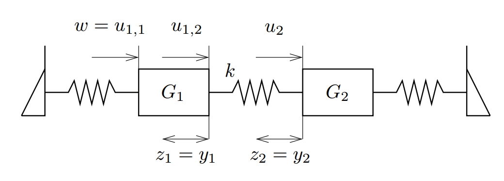
The code used to create the subsystems in the article has been made available for this example and is used to create an instance of ‘SystemNetwork’ that describes the mechanical system. Note that the interconnections in this example contain scalar weights in the form of a spring constant. A special syntax, explained in section 2.1, can be used to add the weights to the connections when creating the instance. The following code will create an interconnected system that describes the given mechanical system:

% Spring-mass-damper system 1
K1 = [40 30 20]; % Internal spring constants
Kwall1 = 50; % Connected to a wall. Gives frame of reference.
K1 = [Kwall1 K1 0];
m1 = [1 1 1 1]; % mass
d1 = [0.1 0.1 0.1 0.1]; % damping
n1 = length(m1); % nbr masses
M1 = blkdiag(eye(n1),diag(m1));

Omegasqr1 = -diag(K1(1:(end-1))) - diag(K1(2:end)) + diag(K1(2:(end-1)),1) + diag(K1(2:(end-1)),-1);
A1 = M1\[zeros(n1,n1) eye(n1) ; Omegasqr1 -diag(d1)];
B1 = [zeros(n1,n1) ; eye(n1)];
B1 = B1(:,[1 end]); % Pick out only "external" forces
C1 = [eye(n1) zeros(n1,n1)];
C1 = C1(end,:); % Pick out only "end" positions
D1 = [0 0];
G1 = ss(A1,B1,C1,D1);

% Spring-mass-damper system 2, connected to a wall
K2 = [20 30 40 50]; % Internal spring constants
Kwall2 = 60; % Connected to a wall. Gives frame of reference.
K2 = [0 K2 Kwall2];
m2 = [1 1 1 1 1]; % mass
d2 = [0.1 0.1 0.1 0.1 0.1]; % damping
n2 = length(m2); % nbr masses
M2 = blkdiag(eye(n2),diag(m2));

Omegasqr2 = -diag(K2(1:(end-1))) - diag(K2(2:end)) + diag(K2(2:(end-1)),1) + diag(K2(2:(end-1)),-1);
A2 = M2\[zeros(n2,n2) eye(n2) ; Omegasqr2 -diag(d2)];
B2 = [zeros(n2,n2) ; eye(n2)];
B2 = B2(:,1); % Pick out only "start" forces. End force provided by
% wall only.
C2 = [eye(n2) zeros(n2,n2)];
C2 = C2(1,:); % Pick out only "start" positions
D2 = 0;
G2 = ss(A2,B2,C2,D2);

k = 10; % spring constant

iedges = [1 2 -k; 2 2 k ; 1 3 k ; 2 3 -k];
einedges = [1 1];
eoutedges = [1 1 ; 2 2];
eedges = [];

systemNetwork = SystemNetwork(iedges,einedges,eoutedges,eedges,G1,G2)

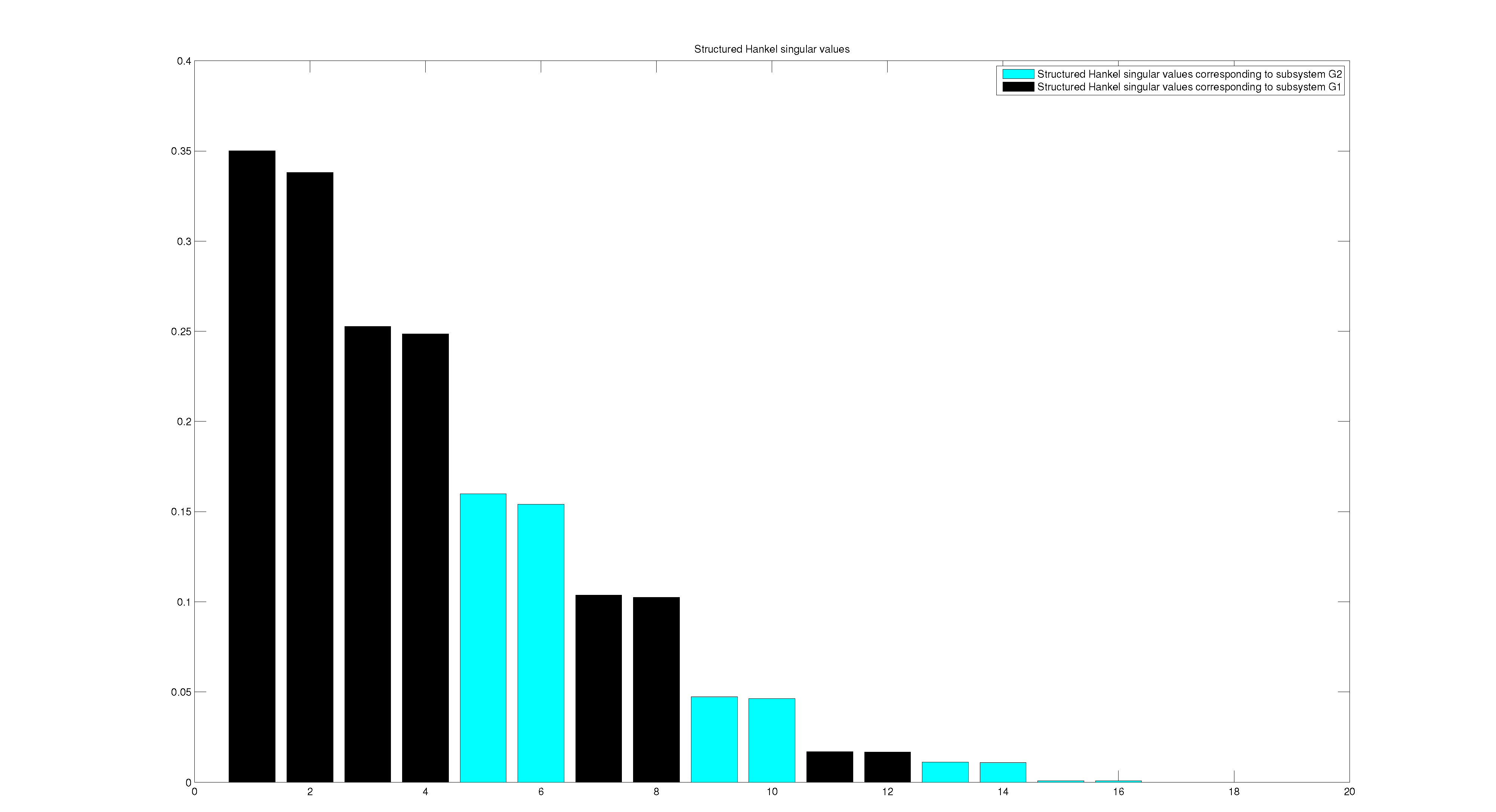
Note that the scalar weight $k$ has been added to the third column of the appropriate edge lists. First, check that the same Hankel singular values as in the article, both regular and structure, are obtained when using the function ‘compareHankels’:

>> compareHankels(systemNetwork)

Figure 9: Structured and unstructured Hankel singular values of the mechanical system.

Close examination upon comparing Fig.9 to Fig.5 in the article confirms that the values obtained in the article are reproduced using the toolbox. Also, if the spring constant is changed from $10$ to $0.1$ , the article calculates structured Hankel values using generalised Gramians. Change $k$ to $0.1$ in the above code and use

>> compareHankels(systemNetwork,’GramianType’,’generalised’)

and observe only the structured Hankel singular values shown in Fig.10

Figure 10: Structured Hankel singular values of the mechanical system, obtained using generalised Gramians.

Upon comparing to rightmost part of Fig.6 in the article, it is evident that the values have been reproduced. Now, attempt to reduce the order of the mechanical system, using balanced reduction:

>> red = balancedNetworkReduction(systemNetwork,[6 6])

and check the

H_{\infty}

error:

>> norm(systemNetwork.structuredRealisation-red.structuredRealisation,inf)
 

 
ans =
 

 
    0.0358

Cross check with table I of the article in the entry where

6

states are kept in each subsystem. Evidently, the toolbox yield the same numerical values.

B ‘SystemNetwork’ Class Reference

B.1 Properties

numberOfNodes: Number of individual subsystems in the structure.

subsystems: Individual state space representation of the systems without the network connections.

The subsystems are stored in a block diagonal form as:

G (s) = (\begin{matrix} G_{1} (s) & 0 \\ ⋱ \\ 0 & G_{n} (s) \end{matrix})

network: Network structure of the system, describing the interconnections

The network of an interconnected linear system is stored as

N = (\begin{matrix} D_{E} & D_{F} \\ D_{H} & D_{K} \end{matrix})

where $D_{K}$ is the adjacency matrix of the internal edges, $D_{H}$ the adjacency matrix of the external inputs to internal inputs, $D_{F}$ the adjacency matrix of the external outputs from internal outputs and $D_{E}$ is the adjacency matrix of the external edges.

structuredRealisation: Structured realisation of the interconnected system $F (N, G)$ .

Given the collection of subsystems $$ \left(\begin{array}{c|c} A_G & B_G \\ \hline C_G & D_G \end{array}\right) \; \text{and the network} \; N = \begin{pmatrix} D_E & D_F \\ D_H & D_K \end{pmatrix} $$

The structured realisation $$ F(N,G) := \left(\begin{array}{c|c} A & B \\ \hline C & D \end{array}\right) = \left(\begin{array}{c|c} A_G+B_GMD_KC_G & B_GMD_H \\ \hline D_FLC_G & D_E+D_FD_GMD_H \end{array}\right) $$

where

L : = {(I - D_{G} D_{K})}^{- 1}, M : = {(I - D_{K} D_{G})}^{- 1}

controlGramian: Controllability Gramian

observeGramian: Observability Gramian

gramianType: Keeps track of the Gramian type

The following types are available:

“uncalculated” - No Gramians have been calculated.
“regular” - Regular Gramians have been calculated.
“generalised” - Structured Gramians have been calculated.
“reserved” - Calculated Gramians are protected from being overwritten by other methods.

B.2 Class constructor

Summary: Constructs an instance of the class ‘SystemNetwork’.

Syntax: systemNetwork = SystemNetwork(internalEdges,externalInputEdges, externalOutputEdges,externalEdges,G1,...,Gn)

Description: An instance of an interconnected linear system is created by supplying a collection of subsystems and $4$ edge-lists that describe the connections in the structure. A detailed example of class construction can be found in section 2.1.

Input
arguments: internalEdges: An edge list of the internal connections where the outputs and inputs of the subsystems have been labelled in consecutive order. A row in the edge list has the format

(e d g e F r o m, e d g e T o)

which implies an edge between the node “edgeFrom” and the node “edgeTo”. A scalar weight can be added to the edge using the format

(e d g e F r o m, e d g e T o, w e i g h t)

externalInputEdges: An edge list of the external input connections where the inputs also have been labelled in consecutive order.

externalOutputEdges: An edge list of the external output connections where the outputs also have been labelled in consecutive order.

externalEdges: An edge list of edges between the external inputs and outputs. If no such connections exist, use an empty array.

$G_{1}, \dots, G_{n}$ : Subsystems of the interconnected system. The subsystems have to be linear time- invariant systems and it is important that they are entered in the same order as their inputs and outputs where labelled.

B.3 Methods

B.3.1 changeSubsystems

Summary: Changes the subsystems without changing the internal network.

Syntax: systemNetwork = systemNetwork.changeSubsystems(stateSizes,sys)
systemNetwork = systemNetwork.changeSubsystems(stateSizes,G1,...,Gn)

Description: changeSubsystems(stateSizes,sys) changes the subsystems of $F (N, G)$ into the systems saved in sys.

changeSubsystems(stateSizes,G1,...,Gn) changes the subsystems of $F (N, G)$ into the subsystems stored in $G_{1}, \dots, G_{n}$

The number of subsystems or the total number of inputs and outputs can not be changed as it would not fit the network. Gramians that have been calculated before the change of subsystem will be removed (unless reserved).

Input
arguments: stateSizes: Vector containing the number of states in each new subsystem. element $i$ contains the number of states in subsystem $G_{i}$

sys: LTI system containing the new subsystems in block diagonal form.

$G_{1}, \dots, G_{n}$ : $n$ LTI systems. The new subsystems have to be enter in the same order as the original were entered during class construction.

B.3.2 extractSubsystems

Summary: Extracts a subsystem from the interconnected system.

Syntax: sys = systemNetwork.extractSubsystem(i)

Description: extractSubsystem(i) extracts subsystem $G_{i}$ from the interconnected linear system.

Input
arguments: $i$ : Index of the desired subsystem.

Output
arguments: sys: state space form of an the desired LTI subsystem.

B.3.3 getStateSizes

Summary: Returns the number of states in each subsystem.

Syntax: stateSizes = systemNetwork.getStateSizes

Description: extractSubsystem(i) extracts subsystem $G_{i}$ from the interconnected linear system.

Output
arguments: stateSizes: Vector containing the number of states in each new subsystem. element $i$ contains the number of states in subsystem $G_{i}$

B.3.4 computeGramians

Summary: Calculates the controllabillity and observability Gramians for the interconnected system.

Syntax: systemNetwork = systemNetwork.computeGramians

Description: The Gramians are solutions to the Lyapunov equations

$A P + P A^{T} + B B^{T} = 0 a n d A^{T} Q + Q A + C^{T} C = 0$

Here, $(A, B, C, D)$ represent the structured realisation $F (N, G)$ of the interconnected system. The resulting Gramians are stored in the properties “controlGramian” and “observeGramian”. The subgramians $P_{i}$ and $Q_{i}$ give information about subsystem $G_{i}$ in relation to the network and they can be extracted using “extractSubgramians”.

B.3.5 computeGeneralisedGramians

Summary: Determines structured Gramians, if they exist, for the interconnected system.

Syntax: systemNetwork = systemNetwork.computeGramians

Description: The method tries to solve the problems

\begin{aligned} min_{P} & t r a c e (P) \\ s.t & A P + P^{T} + B B^{T} < 0 \\ P = diag (P_{1}, \dots, P_{n}) \end{aligned}

\begin{aligned} min_{Q} & t r a c e (Q) \\ s.t & A^{T} Q + Q A + C^{T} C < 0 \\ Q = diag (Q_{1}, \dots, Q_{n}) \end{aligned}

Generalized Gramians that solve these problems are called structured Gramians since they exhibit the same block diagonal form as the subsystems of

F (N, G)

. Structured Gramians do not generally exist. If solutions exist, the resulting Gramians are stored in the properties “controlGramian” and “observeGramian”. If the solver does not find a solution an error message will be displayed and structured Gramians might not exist. The theory of structured Gramians is described in more detail in [2]. Large systems will be cumbersome for the solver and the method is then not recommended for use.

B.3.6 extractSubgramians

Summary: Extracts subgramians from the interconnected system.

Syntax: [Pi,Qi] = extractSubgramians(i)

Description: extractSubgramians(i) extracts subgramians $P_{i}$ and $Q_{i}$ , corresponding to subsystem $G_{i}$ , from $F (N, G)$ . Gramians need to be calculated on before hand using any of the methods below. If the Gramians are not calculated the method will display an error message.

Input
arguments: $i$ : Index of the desired subgramians.

Output
arguments: $P_{i}$ : Controllability Gramian of subsystem $G_{i}$ in the network structure

$Q_{i}$ : Observability Gramian of subsystem $G_{i}$ in the network structure

B.3.7 structuredTransformation

Summary: Performs a transformation that preserves the structure of the interconnected system.

Syntax: systemNetwork = systemNetwork.structuredTransformation(T,redSizes)
systemNetwork = systemNetwork.structuredTransformation(TL,TR,redSizes)

Description: A structured coordinate transformation has the form

T = diag (T_{1}, . . ., T_{n})

$T_{i}$ is an $(n_{i}, n_{i})$ matrix where $n_{i}$ is the size of subsystem $G_{i}$ and $T$ is invertible. A structured coordinate transformation will preserve the internal structure of the interconnected system.

structuredTransformation(T,redSizes) transforms the structured realisation \[F(N,G) := \left(\begin{array}{c|c} A & B \\ \hline C & D \end{array}\right) \; \text{into} \; \left(\begin{array}{c|c} TAT^{-1} & TB \\ \hline CT^{-1} & D \end{array}\right)\]

$T$ needs to have the structure above. If the transformation also reduces the size of $F (N, G)$ through projection, supply the size of subsystem $G_{i}$ in redSizes(i). Otherwise, let “redSizes” be an empty matrix.

structuredTransformation(TL,TR,redSizes) transforms the structured realisation \[F(N,G) := \left(\begin{array}{c|c} A & B \\ \hline C & D \end{array}\right) \; \text{into} \; \left(\begin{array}{c|c} T_LAT_R & T_LB \\ \hline CT_R & D \end{array}\right)\]

Use this version of the method if the right transformation $T_{R} = T^{- 1}$ has already been calculated, to save computation time. $T_{L}$ needs to have the structure above. If the transformation also reduces the size of $F (N, G)$ through projection, supply the size of subsystem $G_{i}$ in redSizes(i). Otherwise, let “redSizes” be an empty matrix.

The method can be used to transform the system into a balanced realization. If the transformation also reduces the system by projection, the reduced size of each subsystem must be supplied in the variable “redSizes”. If the transformation is not a truncation, supply an empty matrix in the “redSizes” field.

Input
arguments: $T$ : Transformation matrix that has to be in the block diagonal form above.

$T_{L}$ : Left transformation matrix that has to be in the block diagonal form above.

$T_{R}$ : Right transformation matrix that has to be the inverse of $T_{L}$

redSizes: Vector containing the number of states in each subsystem after transformation. If the transformation does not reduce the interconnected system, redSizes has to be an empty array.

B.3.8 singularPerturbation

Summary: Performs a singular pertubation of the interconnected system.

Syntax: systemNetwork = systemNetwork.singularPerturbation(redSizes)

Description: Returns an interconnected system where each subsystem has been singularly perturbed and the size of each subsystem after perturbation is stored in “redSizes”. redSizes(i) is the size after perturbation of subsystem $G i$ .

Input
arguments: redSizes: Vector containing the number of states in each subsystem after perturbation

B.3.9 createParametricStructuredRealisation

Summary: Adapter method for genss functions.

Syntax: systemNetwork = systemNetwork.createParametrizedStructuredRealisation
systemNetwork = systemNetwork.createParametrizedStructuredRealisation(i)

Description: createParametrizedStructuredRealisation creates a parametrized version of the interconnected system where all the values in the $A, B, C$ and $D$ matrices in the ss representation of the subsystems are tunable parameters.

createParametrizedStructuredRealisation(i) will only parametrize subsystem $G_{i}$ .

Input
arguments: i: Index of the subsystem that shall be parametrized

B.3.10 generateSimulinkModel

Summary: Generates a Simulink model of the interconnected system.

Syntax: h = systemNetwork.generateSimulinkModel

Description: Returns a handle to the Simulink model with the name “name” and open the simulation. The model includes all the subsystems in the interconnected system connected according to the network $N$ . The input and output ports of the interconnected system are left open and sources and sinks can be connected in relation to the users purpose. An interconnected system with a great number of subsystems and internal connections may not be generated in a readable way and can be troublesome to arrange manually. The method cannot generate the model if several output signals are connected to the same input port. Also, the method does not support scalar weights in the network.

Input
arguments: name: The name of the generated simulation

Output
arguments: h: Handle to the generated simulation.

C Function Reference

C.1 balancedNetworkReduction

Summary: Performs a balanced realisation of an interconnected linear system and reduces the internal subsystems.

Syntax: reducedSystem = balancedNetworkReduction(systemNetwork,redSizes)
reducedSystem = balancedNetworkReduction(systemNetwork,[])
reducedSystem = balancedNetworkReduction(systemNetwork)
reducedSystem = balancedNetworkReduction(systemNetwork,redSizes,options)

Description: A balanced realisation of an interconnected linear system is balanced in the sense of being subsystem balanced. The Gramians $P_{i}$ and $Q_{i}$ corresponding to subsystem $G_{i}$ in a subsystem balanced interconnected system satisfies

P_{i} = Q_{i} = diag (o (i, 1), . . ., o (i, n))

where $o (i, k)$ is the $k$ :th structured Hankel singular value corresponding to subsystem $G_{i}$ . A more detailed definition of subsystem balanced interconnected systems and its implications can be read in [2].

balancedNetworkReduction(systemNetwork,redSizes) will perform a balanced realisation of the interconnected system “systemNetwork”. The interconnected system is an instance of the class ‘SystemNetwork’ The desired size of each subsystem after reduction should be supplied in the array “redSizes” where entry $i$ contains the desired size of subsystem $G_{i}$ after reduction.

balancedNetworkReduction(systemNetwork,[]) If an empty list is supplied instead of “redSizes” the program will show all structured Hankel singular values of the interconnected system, highlight the values corresponding to subsystem $G_{i}$ and prompt the user for the size subsystem $G_{i}$ should be reduced to. The procedure is repeated until reduction-sizes have been chosen for all subsystems.

balancedNetworkReduction(systemNetwork) returns a balanced realisation of “systemNetwork” without reducing the order.

balancedNetworkReduction(network,redSizes,options) specify options for the reduction method.

Input
arguments: systemNetwork: The interconnected linear system that shall be reduced. It has to be an instance of the class ‘SystemNetwork’.

redSizes: Vector containing the number of states in each subsystem after reduction.

options: function-specific options that have to be entered in ‘Key’,‘Value’ pairs. The available options are listed below.

Options: ‘ReductionMethod’:

‘truncation’ - Reduce using truncation (default)
‘perturbation’ - Reduce using singular perturbation

‘GramianType’:

‘regular’ - Use regular Gramians, attained by solving Lyapunov equations (default)
‘generalised’ - Use generalised structured Gramians, attained through solving LMI problems. The existence of such Gramians is not guaranteed.

Output
arguments: reducedSystem: The reduced interconnected linear system. The system is an instance of the class ‘SystemNetwork’.

See also: improveNetworkReduction

C.2 compareHankels

Summary: Compares the structured Hankel singular values of an interconnected linear system to the regular Hankel singular values.

Syntax: compareHankels(systemNetwork)
compareHankels(systemNetwork)

Description: Produces bar plots of the structured Hankel singular values, with values corresponding to each subsystem highlighted. Also, the function plots the regular Hankel singular values of the structured realisation if it treated as one system, with the internal structure being neglected. The aim is to analyse the effect structure has in the interconnected linear system and aid in performing model reduction that preserves the internal structure.

balancedNetworkReduction(network,redSizes,options) specify options for the reduction method.

Input
arguments: systemNetwork: The interconnected linear system that shall be analysed. It has to be an instance of the class ‘SystemNetwork’.

options: function-specific options that have to be entered in ‘Key’,‘Value’ pairs. The available options are listed below.

Options: ‘GramianType’:

‘regular’ - Use regular Gramians, attained by solving Lyapunov equations (default)
‘generalised’ - Use generalised structured Gramians, attained through solving LMI problems. The existence of such Gramians is not guaranteed.

See also: computeStructuredHankels

C.3 computeStructuredHankels

Summary: Calculates the structured Hankel singular values of an interconnected linear system.

Syntax: [hankels,indices] = computeStructuredHankels(systemNetwork)

Description: Returns the structured Hankel singular values of the interconnected linear system. The values are returned in a descending order together with information on which value come from which subsystem. The definition of structured Hankel singular values can be read in [2].

Input
arguments: systemNetwork: The interconnected linear system has to be an instance of the class ‘SystemNetwork’.

Output
arguments: hankels: Vector containing the structured Hankel singular values of the interconnected system in a descending order.

indices: Vector that tracks which subsystem a specific structured Hankel value comes from. The Hankel value stored in hankels(i) originates from the subsystem with the index stored in indices(i).

See also: compareHankels

C.4 improveNetworkReduction

Summary: Tries to improve how well the reduced system approximates the original interconnected linear system.

Syntax: optRed = improveNetworkReduction(originalSystem,reducedSystem)
optRed = improveNetworkReduction(originalSystem,reducedSystem,options)

Description: improveNetworkReduction(originalSystem,reducedSystem) returns a reduced system that better approximates “originalSystem” than “reducedSystem”. The supplied “reducedSystem” should have lower order than the “originalSystem”. The function tries to solve the following optimization problem:

\begin{aligned} min_{G^{'}} & | | F (N, G) - F (N, G^{'}) | |_{\infty} \end{aligned}

where $F (N, G)$ is a structured realisation of the interconnected linear system “originalSystem” and $G^{'}$ is the subsystems of the reduced system. The function will not further reduce the order of the “reducedSystem” but rather alter its parameters so that the $H_{\infty}$ norm of the structured realisations match better. To attain good results, the “reducedSystem” should ideally already have $H_{\infty}$ norm close to the “originalSystem”, for example by utilizing order reduction methods such as balancedNetworkReduction. The function makes use of the “hinfstruct” function to solve the optimization problem.

improveNetworkReduction(originalSystem,reducedSystem,options) specify options for the method as (‘Key’,‘Value’) pairs.

Using the second option ‘parts’ causes the method to solve the following optimization problem:

\begin{aligned} min_{G_{i}^{'}} & | | F (N, G) - F (N, G^{'}) | |_{\infty} \end{aligned}

,where $G^{'}$ consists of the subsystems $(G_{1}, . . ., G_{i}^{'}, . . ., G_{n})$ , for all subsystems $G_{i}^{'}$ . The optimal solution $Ĝ_{i}$ is used when solving the problem with respect to $G_{i + 1}^{'}$ . This version of the solver may not give as good results as solving the whole system at once, but is recommended if the problem is big or takes to long too solve using the ‘complete’ method.

Input
arguments: originalSystem: The interconnected linear system that shall be reduced. It has to be an instance of the class ‘SystemNetwork’.

reducedSystem: The interconnected linear system with reduced order compared to the “originalSystem”. The reduced system is used as a starting guess. It has to be an instance of the class ‘SystemNetwork’.

options: function-specific options that have to be entered in ‘Key’,‘Value’ pairs. The available options are listed below.

Output
arguments: optReducedSystem: The optimally reduced interconnected linear system. The system is an instance of the class ‘SystemNetwork’ and has the same number of states in each subsystem as “reducedSystem”.

Options: ‘SolverMethod’:

‘complete’ - Solves the complete problem as shown above (default)
‘parts’ - Solves the problem in parts, by optimizing with respect to one subsystem at a time, keeping the others constant.

See also: balancedNetworkReduction

Structured ModeL reductIon (SiMpLIfy) Toolbox for MATLAB

Contents

1 Introduction

1.1 Overview of interconnected linear systems

1.2 About the toolbox

1.3 Key features

1.4 Installation

1.5 Requirements

2 Getting started

2.1 Creating an interconnected linear systems

2.2 Using the ‘SystemNetwork’ class features

2.3 Generating a Simulink model

3 Model reduction of an interconnected linear system

3.1 Analysing the system

3.2 Reducing the order of the system

3.3 Improving the model reduction

References

A Examples

A.1 Frequency weighted balanced reduction

A.2 A mechanical example

B ‘SystemNetwork’ Class Reference

B.1 Properties

B.2 Class constructor

B.3 Methods

B.3.1 changeSubsystems

B.3.2 extractSubsystems

B.3.3 getStateSizes

B.3.4 computeGramians

B.3.5 computeGeneralisedGramians

B.3.6 extractSubgramians

B.3.7 structuredTransformation

B.3.8 singularPerturbation

B.3.9 createParametricStructuredRealisation

B.3.10 generateSimulinkModel

C Function Reference

C.1 balancedNetworkReduction

C.2 compareHankels

C.3 computeStructuredHankels

C.4 improveNetworkReduction