CVS revision 1.4
The EDDA documentation system is a collection of scripts created to simplify the process of running ocean simulations and create design documentation.
The system consists of two parts:
Skill scripts to be used in the Cadence OCEAN environment to launch simulations and log simulation results.
The PlainDoc script pddd (based on the pd2tex tool written by Sampo Kellomäki) to capture the simulation results into graphs and tables and create human readable design documentation (HTML and PDF documents).
PlainDoc is a tool to convert text files having a to nicely formatted HTML and PDF documents. PlainDoc is powerfull enough to allows the user to create cross references, insert figures, tables and equations.
An example EDDA design description may look like this.
There are several advantages using the documentation system:
Speed up documentation process. Simulation results are automatically compared to specification and inserted into the simulation document. This minimise the risk of human errors.
Batch simulations over several corners can easily be simulated over night using scripts.
Simple to update results. When a schematic is modified or model file is updated the simulation script can be relaunched and all new results are automatically inserted into the documents.
Both HTML and PDF documents are automatically created for easy sharing of information within design group.
This tutorial is written using PlainDoc by Fredrik Jonsson. You can view the source of this document here.
If you have any comments or suggestions, please contact me at
| (1) |
Also, it would be interresting to know if you sucessfully used EDDA in a project
Click on this link to download EDDA.
Extract the tar file using
> tar -zxvf edda.tar.gz
Copy the file edda/log_data.il to a directory where you store SKILL files, and put the file edda/pddd in your executable search path.
The EDDA system use a number of Unix tools like Perl, LaTeX and image magick when creating the documents. Most of these tools are standard on common Linux distributions. If the tools are not available they have to be downloaded and installed separately.
EDDA have succesfully been tested on sevral different Redhat, Fedora and Cygwin installations.
The EDDA documentation system is created by Fredrik Jonsson.
The EDDA version of PlainDoc is an extension of the PlainDoc tool created by Sampo Kellomäki.
Information about PlainDoc can be found at http://mercnet.pt/plaindoc/pd.html
EDDA is offered under the Gnu Public License (GPL).
Below will follow a short overview how to run simulations and create design documentation using EDDA. In order to use the EDDA system it is assumed you are familiar with running Cadence simulations using Ocean. For information regarding how to configure these tools, please read the cadence documentation.
To create a EDDA document from an existing Cadence simulation testbench we need to:
Create a documentation directory where the simulation files and documents will be generated
Create an OCEAN simulation script file and run the simulations
Create a PlainDoc document
Generate the HTML and PDF documents
The following chapters will explain each step.
Since the EDDA system generates a large number of files the simulations and documents are created in a special directory structure. An example directory looks like figure 1
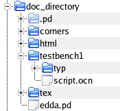
Fig-1: Directory structure
The doc_directory is the documentation directory. This directory can have any name and location.
The .pd directory stores temporary information when running PlainDoc.
corners store files defining the different simulation corners.
html will contain the HTML output
Simulations scripts are stored in testbench directories. The testbench directory contains the netlist and the Ocean scripts. In the testbech directory a subdirectory for each simulation corner will be created containing simulation results. A documentation directory can contain any number of testbenches, but each testbench directory can only have one netlist.
The tex directory contains temporary data when creating a PDF document using LaTeX.
Finally edda.pd is the document source file. The generated HTML and PDF documents will have the same name as the source file.
The directory structure can be generated using the command:
> pddd -init
When running a cadence within the Virtuoso analog design environment you can create an OCEAN script using the menu command Session->Save Script ...
In order to use the OCEAN script in the EDDA environment you need to modify the script according to the following steps:
Move corner definitions to a corner file
Create a symbolic link to the netlist in the testbench directory
Remove information regarding simulator and result directory
Add commands to log simulation results
The steps will be described in more detail below:
A typical automatic generated OCEAN script can look like this:
ocnWaveformTool( 'wavescan )
simulator( 'spectre )
design( "/home/fjon/simulation/simple/spectre/schematic/netlist/netlist")
resultsDir( "/home/fjon/simulation/simple/spectre/schematic" )
modelFile(
    '("/pkg/designkits/umc/MM018/MM180_REG18_V123.lib.scs" "tt")
)
analysis('ac ?start "1k"  ?stop "100M"  )
analysis('dc ?saveOppoint t  )
desVar(	  "Vsupply" 1.8	)
temp( 27 )
run()
ACmag = dB20(VF("/out"))
plot( ACmag ?expr '( "ACmag" ) )
Vdc = VDC("/out")
plot( Vdc ?expr '( "Vdc" ) )
This example script run an simple AC and a DC simulation and plots the result. We will now copy this file to the testbench directory and modify it to be compatible with EDDA.
In order to use the script in the EDDA environment we first extract the corner definition. The corner definition files are located in the corners directory. The corner file can have any name, but the the name typ is reserved for the typical corner.
Extracting the corner information from the example OCEAN file into a corner file. The final file corners/typ may look like this:
 modelFile(
     '("/pkg/designkits/umc/MM018/MM180_REG18_V123.lib.scs" "tt")
 )
 desVar("Vsupply" 1.8)
 temp( 27 )
The sim script will look for a link to the netlist in the test bench directory. When not using EDDA the design will be loaded using the line
design( "/home/fjon/simulation/simple/spectre/schematic/netlist/netlist")
in the ocean script. The actual location of the design file of course depend on the cadence configuration and the user. The design definition must be removed from the script file and be replaced by a symbolic link.
The symbolic link is created using the Unix command
 > cd testbench1
 > ln -s home/fjon/simulation/simple/spectre/schematic/netlist/netlist .
Don't forget the . at the end of the line.
The sim script automatically configures the simulator and results directory so this information can be removed from the scripts file.
Remove the lines
 ocnWaveformTool( 'wavescan )
 simulator( 'spectre )
 design( "/home/fjon/simulation/simple/spectre/schematic/netlist/netlist")
 resultsDir( "/home/fjon/simulation/simple/spectre/schematic" )
from the script file.
The sim script will use the directory /tmp/USER/simulation/SCRIPT to store simulation results, where USER and SCRIPT will be replaced by the user name and name of the script file.
The EDDA system have a set of skill functions to log simulation results. Scalar data can be stored using log_data and waveforms are stored using log_wave. Data from simulation loops can be combined to generate a waveform using log_data_point.
The simulation results are stored as text files within the testbench directory. A subdirectory for each corner will be generated.
To log the DC voltage and the AC response in the example ocean script we can use the following lines:
 log_data(VDC("/out") "Vdc")
 log_wave(dB20(VF("/out")) "ACmag")
If simulation is performed using these commands in the typ corner the files testbench1/typ/Vdc and testbench1/typ/ACmag will be created.
Plot commands from the original ocean script can be removed.
Now all the modifications to the script file is ready and the final script testbench1/script.ocn may look like this:
analysis('ac ?start "1k"  ?stop "100M"  )
analysis('dc ?saveOppoint t  )

run()

log_data(VDC("/out") "Vdc")
log_wave(dB20(VF("/out")) "ACmag")
The simulation script are simulated using ocean. Start ocean within the testbench directory.
 > cd testbench1
 > ocean
Load the EDDA skill functions using
> load "log_data.il"
Now we can run the simulation using
> sim "script.ocn"
If we don't specify a corner the default corner "typ" will be used. To specify another corner we can type
> sim "script.ocn" "fast"
Assuming we have a cornerfile named "fast" in the corners directory.
If the schematic is modified we recreate the netlist from Analog artist using the menu Simulation->Netlist->Recreate
To rerun the simulation script using the previous script file and corner it is enough to type
> sim
A batch simulation simulating many corners can be created, for example by creating a file all containing the lines
 sim "script.ocn" "typ"
 sim "script.ocn" "fast"
 sim "script.ocn" "slow"
and simulating this file using
sim "all"
will simulate over corners typ, fast and slow.
The simulation results can be documented in a design document. The document is written in PlainDoc which is a simple text-file containing a few special "tags" to include simulation results, plots, equations, schematics etc.
In the document we first insert the document title:
 Example simulation
 ##################
After this we insert information indicating the paper format, information about the author etc:
 <<class: article!a4paper,12pt>>
 <<author: Fredrik Jonsson>>
Plain doc use a very simple yet powerful markup structure. Different headings are indicated by the way they are underlined:
 1 Heading 1
 ===========

 1.1 Heading 2
 -------------

 1.1.1 Heading 3
 ~~~~~~~~~~~~~~~
The numbers at the beginning of the line are ignored when compiling the document, and sections are renumbered automatically.
Lists is created by inserting a * or a number at the beginning of a line
 * Bulted list

 1. Numbered list
 2. Item 2
Bold italic and computer output is created by inserting *+ or ~ around a word:
*Bold* +italic+ and ~computer~ output.
Verbatim text blocks
Verbatim text
is created by inserting a single space at the beginning of a line.
Lines beginning with a % are commented out and will not be included in the output documents.
For more detailed information about the PlainDoc syntax, please see the appendix or the PlainDoc documentation.
Simulation results are inserted using the tags data and plot.
Scalar data is inserted into a table like table 1
| Parameter | Spec | Result | Unit | Pass | ||||
|---|---|---|---|---|---|---|---|---|
| Min | Typ | Max | Min | Typ | Max | |||
| DC voltage | 0.7 | 0.9 | 1.1 | 0.80 (slow) | 0.90 | 1.00 (fast) | V | |
using the data command:
The slow and fast tags indicates in which corner the simulation result was found.
To insert the DC voltage from the previous simulation we can use the following lines:
 <<data:Simulation result summary:result1
 dir=testbench1
 Vdc,DC voltage,minmax,0.7,0.9,1.1,V,2
 >>
The first line
<<data:Simulation result summary:result1
specifies the beginning of a data section. The "Simulation result summary" is the caption of the table, and "result1" is a tag that can be used to reference the table.
The next line
dir=testbench1
specifies from which directory the results will be picked. If this line is omitted all directories will be scanned for simulation results.
The line
Vdc,DC voltage,minmax,0.7,0.9,1.1,V,2
specifies data, unit and limits according to the syntax:
Variable, Caption, Spectype, Min, Typ, Max, Unit, Precision
Variable is the name of the variable specified in script file to store the data. The data table can contain any number of variable specifications.
Caption is a short text describing the variable.
Spectype specifies how the results will be compared to the specification. Currently only the spectype minmax is allowed.
min, typ, max is the specification. Simulation results will be compared to these values, and if outside the limit the label "FAIL" will be written in the Pass column. If a parameter have no specification the specification field can be left blank, however the comma signs must not be removed
Unit specifies the unit of the parameters. Values are automatically scaled according to the unit prefix. If we for example specifies the unit to mV the simulated result will be multiplied by a factor 1000 before inserted into the table. Specification values are not scaled and should be specified in the correct unit, i.e. if the limit is 42mV we should use 42 in the specification.
Precision specifies the numerical precision in the tabled.
Plots like the one in figure 2 are inserted using the command plot
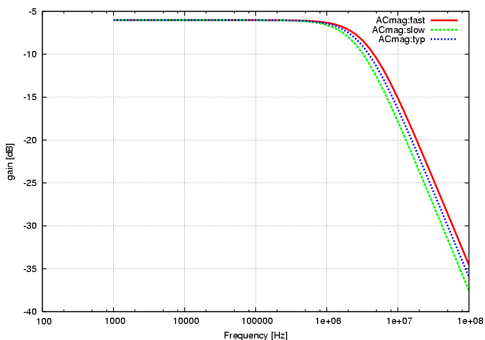
Fig-2: AC gain
The plots are created using gnuplot. By clicking on a plot in the HTML document a magnified version of the graph is presented.
To plot the AC magnitude in the example simulation we use the following line:
 <<plot:
 set logscale x
 ACmag,AC gain,Frequency [Hz],gain [dB],linewidth 5
 >>
The syntax of the plot command is:
waveform(s), Title, X label, Y label, Plot option
waveform is the waveforms to be plotted.
Title is the title of the plot
X axis and Y axis is the labels on the x and y axis.
The set and Plot option commands can be used to specify plot options in gnuplot. All Gnuplot set and unset commands can be used to control the graph. Another useful set command is
set xrange [10:100]
that can be used to control the range on the axis.
For more details regarding available set commands, please refer to the Gnuplot documentation at http://www.gnuplot.info/
Several plots can be specified in one plot statement by adding plot specifications. Set commands must be specified for each plot.
Several waveforms can be plotted in the same graph by putting an & between the plot names. No space is allowed between the names. Specific simulation corners can be selected by putting the corner in parenthesis after the waveform name. The waveform caption can be specified by putting the caption within "". The corner is omitted from the caption if only simulation result from one corner is found.
Example: The following example creates two plots. The first plot (Figure 3) have two waveforms, the first incluing data from the typ and slow corner and label it "Mag" and the second fast corner and label it "Gain fast".
The second plot (Figure 4) is a zoomed in version haing only one wave from the slow corner.
 <<plot:
 set logscale x
 ACmag(typ slow)"Mag"&ACmag(fast)"Gain fast",AC gain,Freq,gain

 set logscale x
 set xrange [1e5:1e7]
 ACmag(slow)"Gain",AC gain,Freq [Hz],gain [dB]
 >>

Fig-3: AC gain
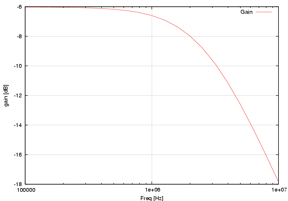
Fig-4: AC gain
By default simulation data from all available corners and testbench directories are collected. You can specify a specific corner or directory by inserting dir and corners lines the same way as in the data table.
If we only want the typ corner from testbench1 we can write:
 dir=testbench1
 corners=typ
The HTML and DPF outputs are generated using the command
> pddd example.pd
The HTML document by viewed by opening the file html/index.html in a web browser. The PDF document is copied both to the HTML directory and to the documentation directory.
An example EDDA design description may look like this. The document is generated using the following source file.
It is sometime useful to include design variables in the design documentation.
Design variables are included using the command
<<desvar:testbench1/script.ocn>>
The command extracts lines containing
desVar("variable" Value); Comment
and creates a table
| Variable | Value | Comment |
|---|---|---|
| Vsupply | 1.8 | Supply voltage |
| c1 | 100p | Parasitic load |
The variables are automatically extracted from an ocean script file. Only variable definitions printed at the beginning of a line will be included. This is in order to allow variables to be omitted from a table by simply adding a space in front of the variable name.
Output log-files can be inserted using
<<logfile:filename.txt>>
The log file is formatted using typewriter type font. Long lines are broken in order to not overflow the paper.
Schematics are included using
 <<sch:
 Schematic (Library)
 >>
where Schematic is the name of the schematic and Library is the library name. You currently have to specify the name of each schematic and library manually.
Schematics should be printed using hierarchical print from cadence to the directory sch in the documentation directory. Plot the schematics without header and remember the last / when specifying the plot path.
Figures and images are inserted using the command
<<img:image, position, size:Caption>>
where image is the name of the image without suffix specifying file type. .eps, .png, and .jpg images are recognised automatically.
The optional position and size are used to control the position and size of the image in the PDF output. Please consult the PlainDoc documentation for details.
Caption is the caption of the image.
Images can be referenced using the image name.
Currently all images have to be located in the documentation directory, including images fron sub-directories do not work.
Example:
<<img:hotdogs.jpg,,3:Hot dogs>>
includes the file hotdogs.jpg from the documentation directory.
Fig-5: Hot dogs
The size "3" makes the image fill 1/3 of the page width in the PDF document.
Tables are inserted using the table command:
 <<table:Example table
 Title1  Title2
 ======= ======
 Text    Value
 >>
Will insert a table:
Table 2:Example table
| Title1 | Title2 |
|---|---|
| Text | Value |
Equations are inserted using the eqn tag.
Syntax:
<<eqn:equation:tag>>
equation is the equation definition using TeX syntax. There are numerous sources of information regarding TeX on the internet. one good starting point is
http://www.artofproblemsolving.com/LaTeX/AoPS_L_GuideCommands.php
tag is an optional tag in order to allow referencing of the equation.
Example:
<<eqn:f_0=\frac{1}{2\pi\sqrt{L(C_0+C_{ext})}}:f_res>>
Generates the equation
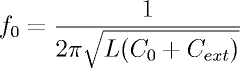 | (2) |
The see command is used to insert a reference
< <see : tag> >
The tag is replaced by the number of the figure, plot or table.
Referencing is done by name matching, where the tag that have the closest match is used. If the match is not exact a warning is generated when generating the document but the reference is still valid.
The skill scripts are a collection of scripts to launch simulations and to log simulation results. These scripts are used as commands within an ocean script.
Table 3 lists the available skill scripts.
Table 3:Skill scripts
| Script | Description | Reference |
|---|---|---|
| sim | Launch a simulation | 4.2.1 |
| log_data | Log data point | 4.2.2 |
| log_wave | Log waveform | 4.2.3 |
| log_data_point | Creates waveform from data points | 4.2.4 |
| log_data_gap | Creates a gap in a waveform | 4.2.5 |
Load simulation script and run simulation.
Syntax:
sim "ocean_script" "corner"
Example:
> sim "test.ocn" "slow"
The example above simulates the script test.ocn in corner slow.
> sim "test.ocn"
runs the simulation in the same corner as previous simulation. Default corner is typ.
> sim
repeats the simulation using previous script file and corner.
Log single value data point.
Syntax:
log_data( data "filename" )
Data will be saved in the folder corresponding to the current simulation corner.
Example:
log_data(IDC("/V0/PLUS") "Isupply")
Log waveform data
Syntax:
log_wave( waveform "filename")
Save waveform data to a file named filename. Data will be saved in the folder corresponding to the current simulation corner.
Example:
log_wave(VT("/Vout") "Vout")
Save numerical data-point to waveform file
Syntax:
log_data_point(xdata ydata "filename")
This function is useful in simulation loops, where each iteration creates a new data-point.
Example:
 foreach(vbias '(0.8 0.9 1.0)
   desVar("Vbias" vbias)
   run()
   log_data_point(vbias value(dB20(VF("/out")),10M) "ACgain10M_vs_bias")
 )
runs three simulations for vbias = 0.8, 0.9 and 1.0. A waveform ACgain10M_vs_bias is created.
Lifts the pen in a waveform. Syntax:
log_data_gap(output)
This is useful if the plot should not be a continues line.
Example:
log_data_gap("ACgain10M_vs_bias")
pddd is a pearl script to generate the HTML and PDF files from the PlainDoc document.
 pddd plaindoc.pd : Convert plaindoc.pd to PDF and HTML
 pddd -init       : Creates simulation directories
The pddd script is based on the PlainDoc system script pd2tex originally created by Sampo Kellomäki, but with several extensions and improvements. The modifications was initially only intended for personal use, but as the project grew I decided to make the modifications public. Since documents created for pddd are not fully compatible with pd2tex I decided to make pddd a branch of the PlainDoc project.
The added features do currently not support DBX output.
Table 4:Change log
| Date | Description | rev | User |
|---|---|---|---|
| 2007-10-16 | Image inclusion now possible from sub-directories | 1.4 | F Jonsson |