2.0 Background

2.1 The constituents of memory

During the latter part of the 20^th century, the study of the brain moved from a peripheral position within both the biological and psychological sciences to become an interdisciplinary field called neuroscience that now occupies a central position within each discipline. This realignment occurred because the biological study of the brain became incorporated into a common framework with cell and molecular biology on the one side and with psychology on the other. In recent years, neuroscientists and cognitive psychologists have recognized many important distinctions of different sorts of memory. There is a lot of speculations to how the memory is constructed and what functions it has. Since the memory is a very integrated system, it’s hard to test specific parts / properties of it. The mixture of two disciplines is one of the reasons why there are so many ideas to how the memory is constructed, and the jungle of terminology surrounding the subject.

The different memory systems have been distinguished according to several attributes or criteria. Here are some of the more important differences; The content or kind of information those systems mediate and store (Episodic / Semantic / Procedural memory) and how they store and retrieve that information (Explicit / Implicit memory). Another distinction is the memory’s storage capacity and the duration of the information storage (LTM / STM).

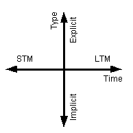
Figure 1 An illustration of how the properties of memory can viewed to be orthogonal. The horizontal axis represents the time span of the memories and the vertical axis could be said to represent awareness of the memories.

2.1.1 Long- and short-term memory

LTM can be thought of as a sturdy memory with almost unlimited capacity. The LTM is thought to reside in the different receptive areas of the cerebral cortex [11]. A closer description of the receptive areas of the cerebral cortex is presented in section 2.2. LTM can be seen to be composed of two different types of memory, declarative memories and nondeclarative memories. An example of declarative memory is the name of your mother, while your cycling skill is a nondeclarative memory. The time scale for long-term memory operations ranges from minutes to years. The time span of a memory depends on a number of factors. One of the most important factors is the number of times the memory is presented to you.

The concept of a STM has been around for a long time. The time scale of short-term memory operations ranges from less than a second to minutes. It’s an appealing idea that it exists some sort of temporary memory storage where sensory impressions could temporarily be stored before they are processed or before they become consolidated into LTM. Several kinds of STM have been described, again mainly on the basis of storage-time distinctions and phenomenal or neuropsychological data. The shortest of STM would be iconic memory [12], which has the capacity to retain a visual image for up to 1 second after presentation. Echoic memory is used to store sounds, and has a slightly longer time span then iconic memory. Immediate memory would last a few seconds longer. Although different STM have been proposed, I will not deepen the discussion into the subject of different kinds of STM, instead I will adapt a broader view of the subject.

The definition of STM that transcends the temporal criterion is working memory. Working memory is a concept of STM that derives from cognitive psychology [8]. Working memory is thought to be a temporary storage used in performance of cognitive behavioural tasks, such as reading, problem solving, and delay tasks (e.g., delayed response and delayed matching to sample), all of which require the integration of temporally separate items of information. Baddeley have more recently developed his view of working memory, and he now states that it constitutes of a phonological loop, a visuospatial sketchpad and the central executive [8].

2.1.2 Explicit and implicit memory

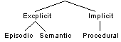
Figure 2 A hierarchic view of the constituents of explicit and implicit memory. Explicit memories, are memories that you are aware of. Implicit memories are memories you possess, but are not aware of. Explicit memories can be divided into two categories, episodic and semantic memories. Episodic memories are whole scenarios. Semantic memories are lexical memories i.e. words. A form of implicit memory is procedural memory. As mentioned earlier, the group of implicit memories are memories you are not aware of i.e. the skill of cycling.

Explicit (or declarative) memory is the memory of events and facts; it is what is commonly understood as personal memory. One part of it contains the temporally and spatially encoded events of the subject’s life for which reason it has alternately been called episodic memory [13, 14]. Another part contains the knowledge of facts that are no longer ascribable to any particular occasion in life; they are facts that, through single or repeated encounters, the subject has come to categorize as concepts, abstractions, and evidence of reality, without necessarily remembering when or where he or she acquired it. This is what Tulving has called semantic memory [14].

Implicit (or nondeclarative) memory, the counterpart of declarative memory, is a somewhat difficult concept to grasp. It can be viewed as the memory for development of motor skills although it encompasses a wide variety of skills and mental operations. Cohen and Squire called this type of memory procedural memory [15]. Implicit memory can also be viewed as the influence of recent experiences on behaviour, even though the recent experiences are not explicitly remembered. For example, if you have been reading the newspaper while ignoring a television talk show, you may not explicitly remember any of the words that they used in the talk show. But in a later discussion, you will more likely use the words that they used in the talk show. Psychologists call this phenomenon priming, because hearing certain words “primes” you to use them yourself.

2.2 The nervous system

The nervous system consists of the central nervous system and the peripheral nervous system. The central nervous system (CSN) is the spinal cord and the brain, which in turn include a great many substructures. The peripheral nervous system (PNS) has two divisions: the somatic nervous system, which consists of the nerves that convey messages from the sense organs to the CNS and from the CNS to the muscles and glands, and the autonomic nervous system, a set of neurons that control the heart, the intestines and other organs.

The brain is the major component of the nervous system and it is a complex piece of “hardware”. Weighing approximately 1.4 kilogram in an adult human, it consists of more than 10¹⁰ neurons and approximately 6*10¹³ connections between these neurons [16]. The struggle to understand the brain has been made easier because of the pioneering work of Ramón y Cajál [17], who introduced the idea of neurons as structural constituents of the brain. I will now make some comparisons that are far from valid but although quite illustrative. Typically, neurons are five to six orders of magnitude slower than silicon logic gates; events in a silicon chip happen in the nanosecond (10^-9 s) range, whereas neural events happen in the millisecond (10^-3 s) range. However, the brain makes up for the relatively slow rate of operation of a neuron by having a truly staggering number of neurons with massive interconnections between them. Although the brain constitutes an incredibly large number of neurons, it’s still very energy efficient. The brain use approximately 10^-16 joules per operation per second, whereas the corresponding value for the computers in use today is about 10^-6 joules per operation per second [18]. If one makes the assumption that the brain consumes 400 kg-calories/24h, the brain has an effect of 20 watts, which is equal to a modern processor.

2.2.1 Nerve cells

What sets neurons apart from other cells are their shape and their ability to convey electrical signals. The anatomy of a neuron can be divided into three major components: the soma (cell body), dendrites and an axon. The soma contains a nucleus, mitochondria, ribosomes and the other structures typical of animal cells. Neurons come in a wide variety of shapes and sizes in different parts of the brain. The pyramidal cell is one of the most common types of cortical neurons. The typical pyramidal cell can receive more than 10,000 synaptic contacts, and it can project onto thousands of target cells. Axons are the transmission lines from the soma to the synapse, and dendrites are the transmission lines from the synapses to the soma. These two types of cell filaments are often distinguished on a morphological ground. An axon often has few branches and greater length, whereas a dendrite has more branches and shorter length. There are some exceptions to this view. Some dendrites contain dendritic spines where specialized axons can attach [19].

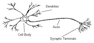
Figure 3 A pyramidal cell, which is the most common type of nerve cell in the cerebral cortex. The pyramidal cell is here depicted with only its most important filaments, the dendrites, the axon with its synaptic terminals, and the cell body. [Figure 3]

Synapses are elementary structural and functional units that mediate the interactions between neurons. The most common kind of synapse is a chemical synapse. A presynaptic process liberates a transmitter substance that diffuses across the synaptic junction between neurons and then acts on a postsynaptic process. Thus a synapse converts a presynaptic electrical signal into a chemical signal and then back again into a postsynaptic electrical signal. It is assumed that a synapse is a simple connection that can impose excitation or inhibition, but not both on the receptive neuron. It is established that the synapses can store information about how easily signals should be able to pass through. The process that account for this ability is LTP (Long Term Potentiation). In the case of inhibitory synapses there is a similar process called LTD (Long Term Depression) [1].

The majority of neurons encode their outputs as a series of brief voltage pulses. These pulses, commonly known as actionpotentials or spikes, originate at or close to the soma (cell body) of neurons and then propagate across the individual neurons at constant velocity and amplitude. The reasons for the use of actionpotentials for communication among neurons are based on the physics of axons. The transportation of the actionpotentials is an active process. The axon is equipped with ion-pumps, that actively transport K⁺, Na²⁺, Cl^-, ions in and out through the axon’s cell membrane. The active transportation of actionpotentials is necessary when the axons span great distances otherwise the actionpotentials would be too reduced. If the actionpotentials are too reduced when they reach the end of the synapses, they are not able to initiate the release of transmitter substances. The myelin or fat that surrounds the axons lessen the reduction of the actionpotentials.

2.2.2 Cerebral cortex

The surface of the forebrain consists of two cerebral hemispheres, one on the left side and one on the right, that surround all the other forebrain structures. Each hemisphere is organized to receive sensory information, mostly from the contralateral side of the body, and to control muscles, mostly on the contralateral side, through axons to the spinal cord and cranial nerve nuclei. The cellular layers on the outer surface of the cerebral hemispheres form grey matter known as the cerebral cortex. Large numbers of axons extend inward from the cortex, forming the white matter of the cerebral hemispheres. Neurons in each hemisphere communicate with neurons in the corresponding part of the other hemisphere through the coreus callosum, a large bundle of axons.

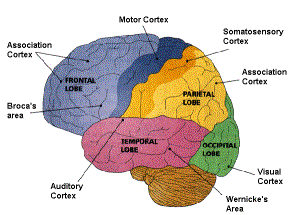
Figure 4 The cerebral cortex of a human brain. In the picture the cortex has been divided into it’s major functional areas. There are descriptions of the cortex, where the cortex is divided into 50 functional areas or more. [Figure 4]

The cerebral cortex has a very versatile functionality. At a glance, the cortex seems to be structurally very uniform. This suggests that the functionality of the cortex is very general, but we know that different areas of the cortex handle specific tasks. This is supported by the fact that microscopic structure of the cells of the cerebral cortex varies substantially from one cortical area to another. The differences in appearance relate to differences in the connections, and hence the function. Much research has been directed toward understanding the relationship between structure and function. The sensory and motor cortical areas have been found to have a hierarchy order. In the case of the sensory cortical areas, there are lots of connections from the higher order sensory areas to the prefrontal cortex. In the case of the motor cortical areas, there are lots of connections leading from the prefrontal cortical area to the higher order motor cortical areas [20].

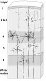
Figure 5 The cerebral cortex is divided into to six layers. Layer 2&3 is often considered as a single layer. There is also a thought of a division of the cortex into columns vertical to the layers of cortex. The existence of these vertical modules is highly debated. [Figure 5]

In humans and most other mammals, the cerebral cortex contains up to six distinct laminas, layers of cell bodies that are parallel to the surface of the cortex. Layers 2 and 3 are usually seen as one layer. Most of the incoming signals arrive in layer 4. The neurons in layer 4 sends most of their output up to layers 2 & 3. Outgoing signals leaves from layers 5 and 6. In the sensory cortical areas the cells or neurons with similar interests tend to be vertically arrayed in the cortex, forming cylinders known as cortical columns. The small structures, called mini-columns, are about 30 mm in diameter. These columns are summed up into larger structures called hypercolumns that are about 0.4 -1.0 mm. In the artificial neural network used to run the simulations described later on, there will be a similar concept to the hypercolumns. Outside the sensory areas the structures of the columns are less distinct. Each column in a hypercolumn can be seen to perform a small and specific piece of the work that is preformed by a hypercolumn. Within a hypercolumn the communication between the columns constituting the hypercolumn, is very intensive [21].

2.3 Computational structures designed to mimic biological neural networks

Neural networks are very interesting, because they work in a completely different way than a conventional digital computer does. Neural networks process information, using a vast number of non-linear computational units. This means that the computations are done in a non-linear and highly parallel manner. A conventional computer, based on the von Neumann machine, often only uses one computational unit, hence process the information in a sequential manner. It is often said that neural networks are superior to the standard von Neumann machines. This isn’t true, but it’s a fact that neural networks and von Neumann machines are good at different forms of computations [22].

The neural networks used in this thesis were implemented on regular desktop computers. This is usually the case, since it’s much easier to construct an implementation in software than in hardware. A hardware implementation of a neural network is more resource efficient.

2.3.1 Different approaches to associative memories

An associative memory is a memory that stores its inputs without labelling them (memories aren’t given an address). To recall a memory you need to present the associative memory with an input similar to the memory you want to retrieve. There are two types of associative memories, auto-associative memories (which are sometimes also referred to as content addressable memories) and hetro-associative memories. When fragmented pattern is presented to an auto-associative memory, the memory tries to complete the pattern. If a fragmented pattern is presented to a hetro-associative memory, the memory tries to associate the presented pattern to another pattern. Note that all the associations are learned in advance [23].

The basic idea behind an auto-associative memory is very simple. Each memory is represented by a pattern. A pattern is a vector containing N binary values corresponding to the states of the N neurons. When an auto-associative memory has been trained with a set of P patterns { x^m } and then presented with a new pattern x^P+1, the auto-associative memory will respond with producing whichever one of the stored patterns most closely resembles x^P+1. This could of course be done with a conventional computer program that computes the Hamming distance between pattern x^P+1 and each of the P stored patterns. The Hamming distance between two binary vectors is the number of bits that are different in the two vectors. But if the patterns are large, and very many (these two attributes usually come together), the auto-associative memory with its highly parallel structure will be immensely faster then the conventional computer program. An example of application is image recognition. Imagine that you receive a very noisy image of your house, if this image previously has been stored in the auto-associative memory, the memory will produce a reconstruction of the image.

Associative memories have more nice features then just noise removal. Associative memories have the very import ability to generalize. This makes it possible for associative memories to handle situations where they are presented with memories never before encountered. Another side of generalization is categorization of memories. This is also a feature handled by associative memories. Categorization means that similar memories are stored as one memory. The common features of the memories, stored in the same category, are stored robustly and are easy to retrieve. The individual details of each memory in the category leave only a minor trace in the memory. When a memory is retrieved from the category, it is very likely to posses the details of the most recently stored memory.

The workings of the associative memory are usually explained by an energy abstraction. In this abstraction, the memories stored in the associative memory, constructs an energy landscape. The energy landscape has as many dimension as the stored memories have attributes. This often means that the energy landscape has a high number of dimensions. The energy landscape in figure 6 only has two dimensions and thus the memories stored, in the corresponding associative memory, only have two attributes. Each learned memory creates a local minimum in the energy landscape. These local minimums are called attractors. In this concept, the input to the associative memory is a position in the energy landscape, where information is stored as a basin in the energy landscape. The retrieval of a memory can be seen as a search for a local minimum in the energy landscape. The starting point for this search is the input, which is similar to the memory that is going to be retrieved. Although this view can be quite elusive, since we are talking about a high dimensional space, it nonetheless gives an illustrative view of the way an associative memory works.

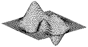
Figure 6 An illustration of the energy landscape that is produced by the associative memory. The basins, the lowest points in this energy landscape, are called attractors. The attractors could be said to constitute the memories in an associative memory. These types of networks are referred to as attractor networks.

There are several ways an associative memory can be constructed. The most common method is to use the Hopfield model to construct an associative memory. In this thesis I will use an advanced version of the Hopfield model, based on the laws of probabilities, to construct associative memories.

2.3.2 The Hopfield model

The idea behind the Hopfield model is largely based on Donald Hebb’s well known work: Assume that we have a set of neurons, which are connected to each other through connection weights (representing synapses) [24]. In the discrete Hopfield model, the neurons can either be active or non-active. When the neurons are stimulated with a pattern of activity, correlated activity causes connection weights between them to grow, strengthening their connections. This makes it easier for neurons that in the past have been associated to activate each other. If the network is trained with a pattern, and then presented with a partial pattern that fits the learned pattern it will stimulate the remaining neurons of the pattern to become active, completing it. If two neurons are anti-correlated (one neuron is active while the other neuron is not) the connection weights between them are weakened or become inhibitory. This form of learning is called Hebbian learning, and is one of the most used non-supervised forms of learning in neural networks.

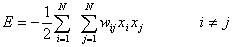
The Hopfield network consists of a set of neurons and a corresponding set of unit delays, forming a multiple-loop feedback system [9]. If N is the number of neurons in the network, the number of feedback loops is equal to N²-N. The ”–N” expression represents the exclusion of self-feedback. Basically, the output of each neuron is fed back, via a unit delay element, to each of the other neurons in the network. Note that the neurons don’t have self-feedback. The reason to this is that self-feedback would create a static network, which in turn means a non-functioning memory.

Each feedback-loop in the Hopfield network is associated with a weight, w_ij. Since we had N²-N feedback loops, we will have N²-N weights. Imagine that we have P patterns, where each pattern, x^m, is a vector containing the values 1 or –1. Then a weight matrix can be constructed in the following manner:

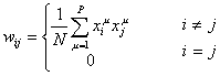
where m is index within a set of patterns, P is the number of patterns, and N is the number of units in a pattern (N is the size of the vectors in the set { x^m }). The patterns represent the activation of the neurons. The neurons can be in the states o_i Î ±1.

To recall a pattern (of activation), o_i, in this network we can use the following update rule:

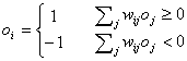
If the underlying network is recurrent the process of recollection is iterative. This iterative process, where the instable and noisy memory becomes stable and clear, is called relaxation.

Since the network will have a symmetric weight matrix, w_ij, its possible to define a energy function called Lyapunov function [25]. The Lyapunov function is a finite-valued function that always decreases as the network changes states during relaxation. According to Lyapunov’s Theorem 1, the function will have a minimum somewhere in the energy landscape, which means the dynamics must end up in an attractor. The Lyapunov function is for a pattern x defined by:

The Hopfield model constitutes a very simple and appealing way to create an associative memory. The model have a problem called catastrophic forgetting. Catastrophic forgetting occurs when the Hopfield network is loaded with too many patterns. It can be said to occur when there are to many basins in the energy landscape. If the network is loaded with to many patterns, errors in the recalled patterns will be very severe. The storage capacity of the Hopfield network is approximately 0.14N patterns, where N is the numbers of neurons in the network [25].

The Hopfield model can also be made continuous. The model is then described by a system of non-linear first-order differential equations. These equations represent a trajectory in state space, which seeks out the minima of the energy (Lyapunov) function E and comes to an asymptotic stop at such fixed points in analogy with discrete Hopfield model presented.

2.3.3 Extensions to the Hopfield model

The standard correlation based learning rule used in the Hopfield model, suffers from catastrophic forgetting. To cope with this situation Nadal, Toulouse and Changeaux [26] proposed a so-called marginalist-learning paradigm where the acquisition intensity is tuned to the present level of cross talk “noise” from other patterns. This makes the most recently learned pattern the most stable. New patterns are stored on top of older ones, which are gradually overwritten and become inaccessible, a so-called “palimpsest memory”. This system retains the capacity to learn at the price of forgetfulness.

Another smoothly forgetting learning scheme is learning with in bounds, where the synaptic weights w_ij are bounded –A £ w_ij £ A. This learning scheme was proposed by Hopfield [9]. The learning rule for training patterns xⁿ is

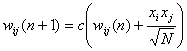
where c is a clipping function

The optimal capacity 0.05N is reached for A » 0.4 [27]. For high values of A, catastrophic forgetting occurs, for low values the network remembers only the most recent pattern. This implies a decrease in storage capacity from 0.14N of the standard Hopfield model. Total capacity has been sacrificed for long-term stability.

2.4 Bayesian attractor networks

As previously discussed, there are several approaches to creating a memory in a neural network context. This thesis uses associative memories with, palimpsest properties and a structure with hypercolumns based on a Bayesian attractor network with incremental learning. This memory model is used because it is a good model of the structures in the cerebral cortex and at the same time comparably simple. The model also makes sense from a statistical viewpoint.

The artificial neural network with hypercolumns and incremental, Bayesian learning developed by Sandberg, et al. [10] is a development of the original Bayesian artificial neural network model developed by Lansner et al. [28-30] , which was developed to be used with one-layer recurrent networks.

The Bayesian learning method is a learning rule intended for units that sum their inputs multiplied by weights and use that sum to determine, by using a non-linear function, their output (activation). This is much like many other algorithms for artificial neural networks. The weights in a Bayesian network are set in accordance with rules derived from Bayes’ expressions concerning conditional probabilities. This means that the unit activation can be equated with the confidence in various features. The rule is local, i.e. it only uses data readily available at either end of a connection. The algorithm allows, in an easy way, to adjust the time span over which statistical data is collected. The time span is adjusted by a single variable, often called a. Regulating the value of a , and hence the time span for collecting statistical data, the plasticity of the network is regulated.

The Bayesian learning rule can be extended to handle continuous valued attributes. This have been done by Holst and Lansner [30], using an extended network capable of handling graded inputs, i.e. probability distributions given as input, and mixture models.

To deal with correlations between units that cause biases in the posterior probability estimates, hypercolumns were introduced [29]. A hypercolumn, named in analogy with cortical hypercolumns [31], is a module of units that represent all possible combinations of values of some primary features and hence provide a anti-correlated representation of the network input.

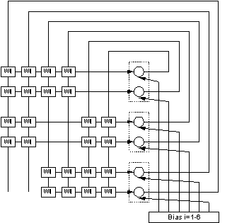
Figure 7 Here is a small recurrent neural network with the 6 neurons divided into three hypercolumns. Note that there are no recurrent connections within each hypercolumn. With some imagination it can also be seen how the weights w_ij form a matrix.

I am now going to present a continuous, incremental Bayesian learning rule with palimpsest memory properties. The forgetfulness can conveniently be regulated by the time constant of the running averages. This implies that we easily can construct a STM or LTM memory with this learning rule.

2.4.1 The Bayesian artificial neural network with incremental learning

Bayesian Confidence Propagation Neural Networks (BCPNN) are based on Hebbian learning and derived from Bayes theorem for conditional probabilities:

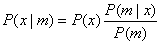
where m is an attribute value of certain class x. The purpose of calculating the probabilities of the observed attributes for each class is to make as few classification errors as possible. The reason we want to use Bayes theorem is that it is often impossible to make a good estimate of P(x|m) directly out of the training data set. On the other hand, a good estimate of P(m|x) is often possible to achieve. Next we will see how this can be implemented in a neural network context.

The input to the network is a binary vector, x. The vector x is composed of the smaller vectors x₁, x₂,…x_N. Each of these sections x₁, x₂,…x_N are representing the input to a hypercolumn. This means that the input space, which represents all possible inputs to the network, can be written as X = X₁, X₂,…X_N

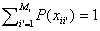
Each variable X_i can take on a set of M_i different values. This means x_i will be composed of M_i binary component attributes x_ii’ (the i’ th possible state of the i th attribute of x_i) with a normalised total probability

From the input, x, we want to estimate the probability of a class or set of attributes y. (The class y is the output of the network and the input, x, is seen as an attribute.) The vector y has the same structure as the vector x. If we condition on X (where unknown attributes retain their prior distributions) and assume the attributes x_i, to be both independent, P(x) = P(x₁)P(x₂)…P(x_N), and conditionally independent, P(x|y) = P(x₁| y)P(x₂| y)…P(x_N| y), we get:

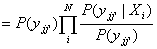
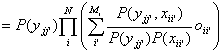
where o_ii’ = P(x_ii’|X_i).

Since y can just be regarded as another random variable it can be included among the attributes x_i and there is no reason to distinguish the case of calculating y_jj’ from calculating x_ii’. If X represents known or estimated information, we want to create a neural network which calculates P(y), from the given information. If we take the logarithm of the above formula we get

(1)

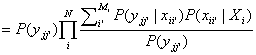
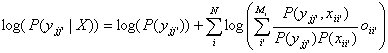
Now, let the input X(t) to the network be viewed as a stochastic process X(t,×) in continuous time. Let X_ii’(t) be component ii’ of X(t), the observed input. Then we can define P_ii’(t)=P{X_ii’(t)=1} and P_ii’jj’(t)=P{X_ii’(t)=1, X_jj’(t)=1}. Equation (1) becomes:

(2)

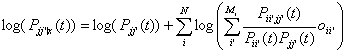
Given the information {X(t’),t’<t} we now want to estimate P_ii’(t) and P_ii’jj’(t). This can be done by using current unit activity o_ii’(n) at time n with the following two estimators where t is a suitable time constant.

(3)

(4)

The estimator in equation (3) estimates the probability of a single neuron to become active per time unit. The estimator in equation (4) estimates the probability for two neurons to simultaneously be active. L is the estimated probability per time unit or rate estimated probability. This means that L is estimated from a subset of the events that has occurred, whereas P is estimated from all events that has occurred. The rate estimator explains the palimpsest property of the learning rule.

These estimates can be combined into a connection weight, which is updated over time. The bias can also easily be stated:

(5)

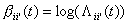(6)

The base for the logarithms is irrelevant, but for performance reasons the natural logarithm is often the best choice. Logarithms with other bases are often derived from the computation of the natural logarithm.

The usual equation for neural network activation is

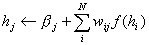(7)

where h_j is the support value of unit j, b_j is its bias, w_ij the weight from i to j and f(h_i) the output of unit i calculated using the transfer function f. The output f(h_i) equals o_ii’ in equation (1) and (2). In the basic Hopfield model the activation function, f(), is, as we earlier saw, a step function.

The form in equation (2) is slightly more involved then (7), and has to be implemented as a pi-s neural network or approximated [29, 30]. The activation equation in the learning rule is

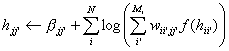(8)

Comparing terms in equation (8) and (2) we make the identifications

(9)

(10)

(11)

P(x_ii’|x) = o_ii’= f(h_ii’) can be identified as the output of unit ii’, the probability that event x_ii’ has occurred or an inference that it has occurred. Since inferences are uncertain, it is reasonable to allow values between zero and one, corresponding to different levels of confidence in x_ii’.

Since the independence assumption is often only approximately fulfilled and we deal with approximations of probability, it is necessary to normalise the output within each hypercolumn:

(12)

The network is used with an encoding mode where the weights are set and a retrieval mode where inferences are made. Input to the network is introduced by setting the activations of the relevant units (representing known events or features). As the network is updated the activation spreads, creating a posterior inferences of the likelihood of other features.

As we discussed earlier, networks with update rules like equation (7) and symmetric weight matrices an energy function can be defined, and convergence to a fixed point is assured [27]. In this case this does not strictly apply, but for activation patterns leaving only one nonzero unit in each hypercolumn, it does apply. In practice it almost always converges, even though there is no input.

In the absence of any information, there is risk for underflow in the calculations. Therefore we introduce a basic low rate l₀. In the absence of signals L_ii’(t) and L_jj’(t) now converges towards l₀ and L_ii’jj’ towards l²₀, producing w_ii’jj’(t) = 1 for large t (corresponding to uncoupled units). The smallest possible weight value if the state variables are initialised to l₀ and l²₀ respectively is 4l²₀, and the smallest possible bias log (l₀). The upper bound on the weights becomes 1/l₀. This learning rule is hence a form of learning within bounds, although in practice the magnitude of the weights rarely comes close to the bounds.

2.4.2 Equations of the incremental, Bayesian learning rule

The learning rule (equations (3)-(6)) of the preceding section can be used in an attractor network similar to the Hopfield model by combining them with an update rule similar to equations (8)-(12). The activities of the units can then be updated using a relaxation scheme (for example by sequentially changing the units with the largest discrepancies between their activity and their support from other units). One could also use a random or synchronous updating similar to an ordinary attractor neural network, moving it towards a more consistent state. This latter approach is used here. The continuous time version of the update and learning rule takes the following form (the discrete version is just a discreteisation of the continuous version using Euler’s method):

(13)

(14)

(15)

(16)

(17)

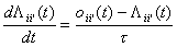
(18)

where t₀ is the time constant of change in unit state. a = 1/t is the inverse of the learning time constant; it is a more convenient parameter than t. By setting a temporarily to zero the network activity can change with no corresponding weight changes, for example during retrieval mode.

The use of hypercolumns in the model presented implies that there will be no recurrent connections within a hypercolumn of the network. Recurrent connections within a hypercolumn are fully anti-correlated. The self-recurrent connection is fully correlated. Thus the weights connecting the neurons within a hypercolumn would either be set to their minimum or their maximum value.

Each neuron in the network will have a bias that is derived from the basic set of recurrent connections. Connections projected from other populations of neurons will not add any bias to the receiving neurons, although it would make sense from a mathematical point of view to include the bias in the projection.

2.4.3 A biological interpretation of the Bayesian Attractor Network

Auto-associative memories based on artificial neural attractor networks, like for example early binary associative memories and the more recent Hopfield net, have been proposed as models for biological associative memory [9, 32]. They can be regarded as formalisations of Donald Hebb’s original ideas of synaptic plasticity and emerging cell assemblies. In this view each neuron in the artificial neural network is thought to equal a single nerve cell in the biological neural network. In figure 8 is an illustration of an artificial neuron. With some imagination it is possible to see the similarities with a nerve cell.

Figure 8 Depicted here is an artificial neuron, and its functions. Some parallels to a biological neuron are inferred in the figure. Note that the output is conveyed to several other neurons.

Each connection weight, w_ij, in figure 8 can be interpreted as a synaptic connection between two neurons. In figure 9 one of these connections is depicted in more detail.

Figure 9 This figure shows a single synaptic connection between two neurons in our artificial neural network. The values of L_i (=P_i, P_j), L_ij (=P_ij), and w_ij , derived in equations (15, 16, 18), can be interpreted as shown in figure. P_j, P_i, P_ij, are values associated with synaptic terminals, synaps, dendrites ability to convey a signal from cell j to cell i.

Although the above presented view of each neuron corresponding to a nerve cell is appealing, it isn’t realistic. Real neurons aren’t as versatile as our artificial neurons i.e. a real neuron can’t impose both inhibition and excitation, which is stated by Dalés law [33]. A better view of the correspondence between our artificial neurons and real neurons is to think of our artificial neurons as corresponding to a cortical column of real neurons. In our Bayesian attractor network we have a structure of hypercolumns, where each hypercolumn is corresponding to a group of cortical columns.

2.5 Interesting concepts

There are a couple interesting concepts or functions I hope to find in the simulations of the memory systems developed in the experiments. These concepts originate from cognitive psychology.

2.5.1 Short-term variable binding

In a memory that’s going to be implemented in a decision making system, there’s a need not only to be able to recall earlier events, but also be able to recall these events with current situation data. This type of process is usually called short-term variable binding (STVB) or role filling. To illustrate this concept I will give an example:

John is visiting his grandfather Sven. After he has visited his grandfather, John meets his two friends, Max and Sven. When Max talks about Sven with John, John knows that the Sven, Max is talking about isn’t his grandfather.

To achieve STVB in a system, the system will of course need a LTM, and also some sort of STM that can accommodate the temporary bindings. One of the main focuses of this thesis will be to investigate how STVB can be achieved.

2.5.2 Chunking

The chunking process is a specialisation of the memory, which allows it to more effectively remember certain things. The chunking learning process recruits a new idea to represent each thought, and strengthens associations in both directions between the new chunk idea and its constituents. Thus, the inventory of ideas in the mind does not remain constant over time, but rather increases due to chunking. The representation of a chunk is constructed out of its constituents. An example of chunking is how the set { 1 2 3 } is remembered. The set can be remembered as 1, 2, and 3. The chunked version of the set is remembered as the number 123.

There are two primary reasons for chunking: First, chunking helps us to overcome the limited attention span of thought by permitting us to represent thoughts of arbitrary complexity of constituent structure by a single (chunk) idea. Second, chunking permits us to have associations to and from a chunk idea that are different from the associations to and from its constituent ideas. This is very important for minimizing associative interference.

In this thesis I have studied how the representation of the short-term memories could be done more effectively. I have also studied how these, efficient short-term representations associates to the long-term representations. Although, the work of this thesis does not directly focus on the chunking process, I thought it was interesting to mention the similarities between the STM & LTM interaction and chunking.

3.0 Method

Since the simulations in this thesis are based upon the Bayesian artificial neural network model developed in [10], I tried to use similar settings and architectures. In all simulations, the neural networks were first trained on a set of patterns, and then tested. This means some consideration must be taken before the artificial neural networks of this thesis can be implemented in a real-time system.

3.1 Design and input

3.1.1 Network and systems

The LTM was implemented as a recurrent network consisting of 100 neurons divided into 10 hypercolumns with 10 neurons in each hypercolumn. This configuration of LTM was used throughout the thesis with no exceptions. As for the STM, there were a couple of different implementations in respect to the number of neurons and of hypercolumns. The two most common implementations of the STM used 100 and 30 neurons respectively. All the networks used, had at least one set of recurrent connections. As earlier mentioned there were no recurrent connections within the hypercolumns of the networks, as the internal representation in a hypercolumn is supposed to be completely anti-correlated.

Almost all systems were constructed under the assumption that the input to the systems always passed the LTM before it entered the STM. The output from the system was always extracted through the LTM. When the systems are used and not only tested, all input/output is handled by the LTM. In a real-time system, the data presented to the STM will always be delayed. Since the simulations in this thesis were not run in real-time, there was no need to be concerned about this delay. The LTM exerted a disruptive influence on the STM during training. The STM exerted a disruptive influence on the LTM during operation. In chapter 5 I investigated these interferences.

The recurrent connection within a network and the connections between networks are called projections. A projection does not only represent the physical connection, the concept also incorporates the connection-weights. Each connection, between two neurons, is equipped with two weights that represent the correlation between the neurons in both directions. Since the networks are auto-associative, the weights are equal in both directions. This does not apply to the connections between two networks, where hetro-associations may arise. In the models, a matrix represents the projections. The bias was not included in the projections.

3.1.2 Input

The input to the artificial neural networks was vectors of binary numbers (0 and 1). These input vectors were constructed in respect to the hypercolumn structure of the LTM. This meant that only one out of ten neurons in a hypercolumn structure was activated and this was always the case. So the whole input of ten hypercolumns only caused 10, out of 100, neurons to be activated. The input could therefore be considered sparse. The sparseness of the input affect the storage capacity of the network. If the input is to “dense”, it will affect the storage capacity negatively. In every run a new set of patterns was generated. The patterns were generated from a rectangular probability-density function.

In chapter 4 the input always consists of sets with 100 patterns. In chapter 5 the input always consists of sets with 50 patterns. Chapter 6 contain experiments with structured data. Therefore the input is sets with different number of patterns. The number of patterns in an input set does not affect the STM since it forgets so quickly. The LTM is affected by the size of the input set. This is more thoroughly explained in 3.2.

3.2 Network operation

As mentioned earlier, the systems designed in this thesis were not operated in “real-time”. The systems had a training mode, where the memories were stored in the system. Then, during operation mode the memories were retrieved. The system design outlined in figure 10 was the most frequently used design. In biological memory systems the theta rhythm may control the switch between training and operation mode of the memory network.

Figure 10 In all simulations, the artificial neural networks were first put in a training mode and were trained with a set of patterns. When the training phase was completed, the networks were put in operation mode, and tested. Note that non-conducting static projections are not depicted in the figure (training mode).

The differential equations 13, 15 and 16 have been solved with Euler’s method. The time-step was chosen to h=0.1, and the integrations lasted for 1 unit of time. (This meant that 10 steps were taken during integration from 0 to 1.) It often took much longer time than one time unit to train or retrieve a pattern properly. In the case of training, a strong memory of a single pattern was achieved trough repeated presentation of the pattern. The relaxation process that occurs during operation mode was almost never fully completed. (Fully completed mean that no more changes would occur if the process was extended.)

3.2.1 Training

During the training mode the equations (15) and (16) were solved for each network in the system. Equations (17) and (18) were then used to compute the bias and the projections for the networks. In the case of projections between two networks, the same equations were applied with the exception of equation (17). The bias was chosen not to be included in the projections between networks. This could of course be discussed. A biological interpretation of this is that the whole dendritic tree of the synapse is given the same bias value. This means that synapses close to the soma are not given any priority. In a real neuron, synapses closer to the soma generate a stronger signal then synapses further out in the dendritic tree [34]. Mathematically it also makes sense to incorporate the bias values into the projection, even though this was not done here.

The three main parameters that controlled the network during training mode were the value of a, the number of patterns and the time spent training each pattern.

3.2.2 Testing

The main interest of this thesis was not the retrieval-performance of the networks. The main interest was to prove that networks with different time-dynamics could be used in the same system. However, retrieval-performance was of great importance when different designs were investigated, to rate how good the designs were.

To initiate the retrieval of patterns (memories) the networks were usually presented with a copy of the learned pattern with 2 errors. (The content of two of the hypercolumns were altered.) In the figures describing the systems, this type of input is denoted as “Input with errors”. In some experiments of chapter 5 and 6 the networks were presented with only a few of the hypercolumns of the learned patterns. The hypercolumns that were not presented to the network were filled with zeros.

The plots over single networks were constructed from 50 runs. In the plots of several networks, each data point was often constructed from 20 runs. The data presented in the tables were accumulated from 100 runs of the networks.

During testing, the networks were put in operation mode. The equation (13) and (14) were used in order to perform the relaxation. The relaxation process was always one time unit long. When a network had a projection from another network, equation (13) was replaced with equation (19). Equation (19) introduces the constant gain factor g. The value of g varied around 1. The purpose of g was to introduce an instrument to control the influence that connected networks imposed on each other. The direction of the projections that g applied to was denoted, i.e. g^STM^®LTM(In this case the connection from the STM to the LTM is scaled with g.)

(19)

Here ws_ii’jj’ denoted the connection-weights and os_jj’ the activity pattern of the sending neurons. Ns is the number neurons in the sending network.

Successful retrieval was defined as the fraction of patterns, which were correctly recalled after relaxation to a tolerance of 0.85 overlap. In the normal case where the input consisted of 10 hypercolumns, a recalled pattern was only allowed to differ in one hypercolumn from the original pattern to be classified as correct. The retrieval ratio of the system was often plotted as a continuous line. The retrieval-ratio of the subsystems were often also plotted, i.e. the LTM (plotted as a dotted line) and the STM (plotted as a dash-dotted line).

3.3 Parameters

In the neural network model at hand there are several parameters that can be chosen more or less arbitrarily. As mentioned earlier, the choice of these parameters is consistent with [10]. In this section the default values of the parameters are listed. These default values are common among many of the simulations. When new constants are introduced or when the default values are altered it has been mentioned it in the text.

In all simulations, the value 0.001 is used for l₀. l₀can be seen as the background noise in the neurons. l₀ also have implications on the maximum excitation that can be conveyed from one neuron to another.

The experiments of chapter 4 were run with 100 patterns. The capacity for an optimal trained LTM with 100 neurons is about 60 patterns. The LTM in the experiments of chapter 4 had a set to a = 0.0005. This low value of a implied that the LTM of chapter 4 could not form properly “deep” attractors after training for 1 unit of time. These two conditions generated a situation where the memories stored in the LTM had a small chance of correct retrieval. Although all trained memories left some sort of trace in the LTM. Chapter 4 investigated the possibility of using a STM to extract those memory traces.

Chapter 5 & 6 contains experiments where the systems where presented with 50 patterns and the LTM was run with a = 0.005. This setting of a allowed the LTM to learn all 50 patterns.

The STM networks in this thesis always had the value of a set a = 0.5. I tried to choose a in such a way that the STM remembered the 10 most recent patterns presented to it. This means that the STM wasn’t affected if the number of patterns presented to it was 50 or 100. Contrary to the LTM of chapter 4, there were no memory traces stored in the STM of the first patterns in the training set.

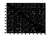
A1 B1 C1

A2 B2 C2

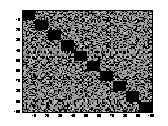
Figure 11 Three connection-weight / projection matrices. .A1 is from a STM. B1 is from a LTM of chapter 5 & 6. C1 is from a LTM of chapter 4. The strength of the connection-weights is colour-coded in A1, B1 and C1 between the logarithmic values 0 and 5. The brighter a dot is, the stronger the connection. The diagonals of the matrices all have black squares, showing the absence of connections within a hypercolumn. A2, B2, C2 are the corresponding distributions of the connection-weights. The vertical line seen in A2, B2, C2 represents the 1000 self-recurrent connection-weights that have been deleted.

There was a difference in the way the projections were set up in a network with a large value of a compared to how the projections were set up in a network with a small value of a. In a net trained with a small value of a (LTM) I found that the distribution of the inhibitory and excitatory weights was very even and distinct. In figure B2 and C2, one can see that the connection-weights are either set to be inhibitory or excitatory. There are not many connection-weights with a value between the two groups of inhibitory and excitatory connection-weights. While in a network trained with a large value of a (STM), the values of the connection-weights were evenly distributed between inhibitory and excitatory connection-weights.

When I coupled a STM to a LTM, the STM memory had an interfering effect on the neurons in the LTM. This meant that the LTM had a smaller probability to relax to the correct pattern. To prohibit this impairment of the LTM, I introduced a gain constant, g^STM^®LTM, between the STM and the LTM (equation (19)). In the systems that were trained with 100 patterns the value of g^STM^®LTM was set to 0.03 and in the systems trained with 50 patterns the g^STM^®LTM was set to 0.1. These values were derived from trial and error processes and they seemed to give the STM a reasonable influence on the LTM.

4.0 Network structures

Chapter 4 investigate the basic concepts of connected networks. In the first part of this chapter, the importance of having recurrent connections with different plasticity kept in different networks (having a separate STM and LTM) is studied. Then, plastic connections are studied. It is also studied how plastic connections can be constructed and used.

The systems in the experiments of this chapter were trained with sets of 100 patterns. The LTM were trained with a set to 0.0005. The LTM had a poor retrieval-ratio of about 0.3. The choice of a meant that all patterns in the training set were remembered, but very poorly.

4.1 Systems with high and low plasticity

The information in a neural network is stored in the projections. Two systems were studied here. The two systems had an equal number of connections, but different number of neurons. N is equal to 100.

The first system, a network of N neurons had two projections with a total of 2N²-20N connections.

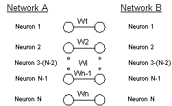
Figure 12 The networks A and B are connected with one-to-one connections. The connection-weights, w_i, were usually set to a value around 10.

The second system had two separate networks, with 2N neurons and 2N²-19N connections. The neurons between these two networks were connected one-to-one projection. This meant that all elements, except the diagonal elements, in the projection matrix were set to 1.

The question was, which of these two systems had the best design. The systems used approximately the same amount of connections. Since memories are stored in the connections, this comparison seemed motivated. (Chapter 5 describes how the design of the second system is made more effective.)

4.1.1 One network with two sets of recurrent connections

Naturally, a neuron takes much more space and uses much more resources than a connection between two neurons. This means that if the number of neurons in a network can be minimized at the expense of more connections in the network, it is a good thing. The system, in this experiment, used few neurons and a moderate number of connections.

Real synapses may posses both low and high plasticity properties. In this experiment the two projections with different plasticity can be seen to form a single projection that have both low and high plasticity properties.

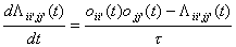
The system was based on a LTM. A “STM” projection^LTM^®LTM with high plasticity was added to the system’s existing “LTM” projection^LTM^®LTM with low plasticity. The high plasticity projection used a set to 0.5 and the low plasticity projection used a set to 0.0005. The bias values were derived from the training of the low plasticity projection, “LTM”. The projection with high plasticity was scaled down with g = 0.03. The value of g was chosen after evaluating the results of the experiment in section 4.2.1. The system was trained with equation (19) instead of equation (13).

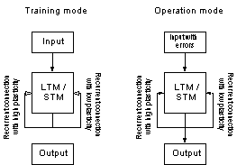
Figure 13 The operation modes of the system. The bias values were derived from the projection with low plasticity. The system was constructed with two projections with different plasticity. Each of the projections, were also treated as individual networks (LTM and STM).

The retrieval-ratio of the system is shown as a solid line in figure 14. The systems two projections, with high and low plasticity were used to create one separate LTM and one separate STM. The separate retrieval-ratio of the LTM is shown as a dotted line, and the retrieval-ratio of the STM is shown as a dash-dotted line, in figure 14. The following text refers to this two (LTM and STM) individualised memories. These two memories were isolated to provide a base for comparison of performance.

The retrieval-ratio of the first 80 patterns was slightly lower for the system than for the LTM. The retrieval-ratio of the last 20 patterns was lower for the system than for the STM. The system seemed to provide compromise of the retrieval-ratio between the LTM and STM. Since the high and low plasticity projections in the system were interacting during the iterative process of relaxation there was a problem with interference between the two projections. The STM interfered the LTM, during retrieval of the first 80 patterns. The STM did not have enough influence over the LTM to control the relaxation process completely, during the last 10 patterns.

It was interesting to see that the system was able to retrieve patterns 85-90 with slightly higher retrieval-ratio than the LTM or STM. During the retrieval of these five patterns the LTM and STM were able to cooperate. This proves that the basic idea of having several projections with different plasticity in a single system can be beneficial.

The compromise between a high retrieval-ratio of the first and the last patterns was controlled by the value of g. Adjustments of g could not improve the projections ability to cooperate. These suggested that this design, with two projections and one population of neurons, was not optimal.

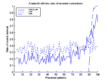
Figure 14 The retrieval-ratio of the system is plotted as continuous line. The retrieval-ratio of the LTM is plotted as a dotted line, and the retrieval-ratio of the STM as a dash-dotted line. Note the increased retrieval-ratio of the system for the last 10 patterns.

4.1.2 Two networks with one set of recurrent connections

This system basically had the same two projections as the system in the previous section. The big difference between the systems was that each of the projections in this system was projected at a separate group of neurons. The purpose of this experiment was to determine if it were beneficial too use two networks with different plasticity.

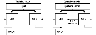
Figure 15 The system has a STM and LTM of equal size. 1-to-1 connections were used to connect the STM to the LTM. The input with errors was fed to both the LTM and STM. Output was extracted from the LTM.

The system was composed a LTM and STM of equal size. These two memories were connected with a 1-to-1 projection^STM^®LTM. The diagonal elements of the projection^STM^®LTM were set to 10. This value was derived from a trial and error process seen in figure 16. When the retrieval-ratio of the system was tested, both of the networks were fed with input.

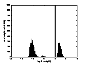
The trail and error process to determine the value of the diagonal elements was performed with ten runs of the system. For each run, the diagonal elements were set to different values. The result of these 10 runs is shown in figure 16. The value of the diagonal elements could have been set to any value between approximately 7-500.

If the diagonal elements, or weights, had been set to one, there would not have been a connection between the two memories. Figure 16 shows this fact. When the weights were set to 1 (equal to 0 on the logarithmic x-axel in figure 16) the retrieval-ratio of the system becomes equal to that of the LTM. And if the weights had been set to a value smaller than one, there would have been an inhibitory effect on the neurons in LTM. If the weights had been set to a value much larger than 500, the system would have shown good performance on the latest learned patterns, but the system would not have been able to recall the patterns learned in the beginning of the training set. This is caused by the strong input from the STM, which makes it impossible for the LTM to relax into a stable state.

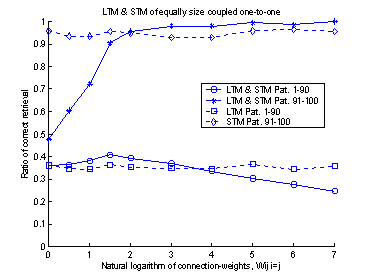
Figure 16 The plot shows 10 runs, with different values of the connection-weights. Performance is measured separately for the first 1-90 patterns and the last 91-100 patterns. The dotted lines represent STM and LTM separately. The solid lines show the performance of the system.

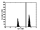
In figure 17 the retrieval-ratio of the system is shown. During the first 80 patterns the retrieval-ratio of the system is equal to that of the LTM. Then, for pattern 80 to 90 the retrieval-ratio is better than both that of the LTM and STM. During the last 10 patterns the retrieval-ratio is equal to that of the STM.

It was interesting to see that the cooperation between the two memories (projections in the previous system) was functioning well. The disruptive influence of the STM on the LTM was almost negligible. The retrieval-ratio of the last 10 patterns was almost 1. A good retrieval-ratio of the most recent patterns is necessary when the STM is to be used as a working memory.

The combination of these facts proved that the design with two individual networks with different plasticity was superior to the design of the system in the previous section.

The STM has a strong influence on the LTM. The STM has the ability to both support and suppress memories in the LTM with great efficiency. This is an important feature, since it provides a way to increase the importance of the latest learned patterns. Later on in this thesis these properties are used to generate useful functions in systems. Systems with STM are designed to prove the possibility of constructing a working memory. The STM also provides the possibility to make reinstatements of the latest memories into the LTM.

Figure 17 A system was based on a STM and LTM of equal size. The STM and LTM were connected with one-to-one connections between the neurons of each network.

4.2 Plastic connections

The experiments presented in this section were designed to investigate how a system built upon two networks, could be connected with plastic projections. Both of the networks, LTM and STM, were of equal size in all the simulations preformed. Different ideas, of how to utilise the plastic projections were investigated.

4.2.1 Plastic connections

There are many connections between the neurons in the cortex, especially between neurons that are close together. It seems very unlikely that these neurons are hardwired and unable to form new connections or delete old connections. In this experiment, the neurons of the two networks (STM & LTM) were allowed to form whatever connections they wanted. As with the recurrent connections, these connections can be made with different plasticity’s.

The connections between the STM and the LTM were in this experiment plastic. The projection^STM^®LTM matrix was no longer diagonal of weights. Instead it was a full matrix of weights, representing all possible wirings between the neurons of the two networks. When the size of the STM differs from that of the LTM or when the pattern representation in the STM differs from that in the LTM, there is a need for a plastic projection. The plastic projections were trained with the same Bayesian learning rule that was used to train the networks recurrent projections. The projection^STM and the projection^STM^®LTM were trained with a set to 0.5. The system’s training and operation mode is seen in figure 18. The projection^STM^®LTM was scaled down with g^STM^®LTM = 0.03.

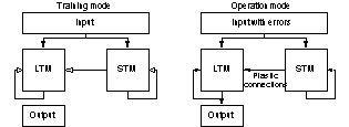
Figure 18 The system used in the experiments of this section. Note the added plastic projection from the STM to the LTM. The plastic projection is a full matrix (100x100) of weights.

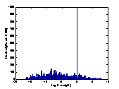
To determine the value of g^STM^®LTM a trial and error process was used. Figure 19 shows 10 runs of the system, with different values of g^STM^®LTM in each run. G was set to the value 0.03 which corresponds to approximately -3.5 on the logarithmic scale of figure 19. If the value of g is set to a smaller value, the retrieval-ratio of patterns 91-100 is decreased. If the g is set to a larger value than 0.03 the retrieval-ratio of patterns 1-90 is decreased. The dotted lines in figure 19 correspond to the performance of a LTM and a STM.

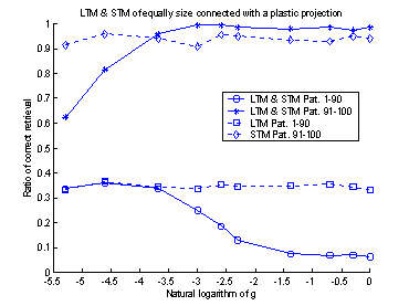
Figure 19 Ten runs of a system with plastic projection. The systems retrieval-ratio is plotted against the logarithmic value of g^STM^®^LTM. An optimum can be found around -3.5. (The exponential of -3.5 is approximately 0.03.) Compare with figure 16.

Figure 20 shows the retrieval-ratio of this system. The performance is very similar to that of the system in section 4.1.2 were we had one-to-one connections. Comparing figure 20 with figure 17, one can se that the projection^STM^®LTM interfere the LTM more then the one-to-one projection^STM^®LTM did. If g^STM^®LTM had been set to 1 this disruptive effect would have been very prominent. The disruptive effect that the STM exerts on the LTM depends on the number of elements that the projection^STM^®LTM contain.

The use of a plastic projection causes a small loss of retrieval-ratio performance, compared to the use of a 1-to-1 projection. This performance loss is compensated by the versatility that the plastic projection provides. Plastic projections allow different representation, of the same data, in the systems different networks. As I later will show, this can generate an increase of the systems performance.

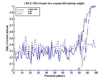
Figure 20 The performance for a system with a plastic connection between a STM and a LTM of equal size. Compare with figure 17.

4.2.2 Sparse plastic connections

Two groups of neurons that are far apart in the brain are usually very sparsely connected. This sounds reasonable since it minimizes the hardware used. It can easily be understood that all neurons in the brain cannot be connected to each other for volume reasons. The experiment I preformed here was aimed at seeking out how the performance is affected when connections between the LTM and STM are deleted.

In the experiment the projection, that connected the STM to the LTM, was made sparse. The sparse projection matrix was achieved through a random deletion of elements (deleted elements were set to 1) in the projection matrix after the projection had been trained. I made 4 runs of the system with different values of g^STM^®LTM in each run.

The influence of the STM on the LTM was reduced when the number of connections was reduced. The influence was then made stronger through an increase of g^STM^®LTM. The correlation between the sparseness of the projection matrix and the value of g^STM^®LTM was of great interest. Figure 21 shows four plots with different values of g^STM^®LTM.

In figure 21A a system with g^STM^®LTM = 0.03 is seen. The systems long-term memory storage capacity was not compromised by the STM. About 40% of the elements in the projection^STM^®LTM could be deleted before the system’s performance was affected. When finally all elements of the projection^STM^®LTM had been deleted, the systems performance was equal to the performance of the LTM alone.

In figure 21B, the value of g^STM^®LTM was increased to 0.1. The increase value of g made it possible to eliminate 60% of all elements in the projection^STM^®LTM without any major loss of performance. The decrease of the performance for the last 10 patterns was steeper then in the previous plots. The plot to the lower left, figure 21C, shows a simulation with g^STM^®LTM = 0.5.

The plot to the lower right, figure 21D shows the performance of the system where g^STM^®LTM was set to 1. The STM suppress the LTM very effectively. Almost all elements in the projection had to be removed before the suppressed retrieval-ratio of the LTM could rise.

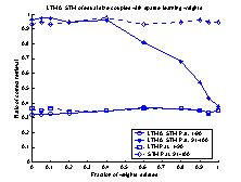
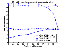
A B

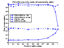
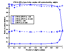
C D

Figure 21 The performance for 4 different values of g^STM^®^LTM. The plot in the upper left have g = 0.03, the plot in the upper right have g = 0.1, the plot in the lower left have g = 0.5 and the plot in the lower right have g = 1. In all of the four plots; in the left side of the plots all connections, between the networks, are present, and to right side of the plots all connections, between the networks, are removed.

It was very interesting to see that more then 60% of the connection could be deleted without any major loss of performance. This provides a hint that it would be possible to shrink the STM without any loss of performance. The most interesting feature of the experiment was that it clearly showed the need to have a scale-factor (g^STM^®LTM) between the connected networks. When g^STM^®LTM is set to 1 it is almost impossible to regulate the influence of the STM on the LTM with the density of elements (connections) in the projection. This is seen in figure 21D. The system, in figure 21D, act either as a STM or as a LTM.

4.2.3 Differently represented patterns in LTM and STM

An interesting question is what happens if the patterns are represented differently in the LTM and the STM. If the connections that provide the LTM with input are different to the ones that provide the input to the STM. In the experiment I studied how the transformation of the patterns affected the performance of the system. Was it possible for the STM and LTM to cooperate with different representation of the memories?

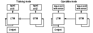
Figure 22 The system used two different sets of patterns. In the experiments I studied how the STM could help the LTM to retrieve the correct patterns, although it had been trained with a different set of patterns.

In the experiment, I produced one set of patterns that I used to train the LTM. I produced another set of patterns that I used to train the STM. The hypercolumn structure of the input patterns existed in both sets of patterns. The projection^STM^®LTM was plastic. The constants of the system were set to the same values as in the previous experiments.

In the experiment the representation of the data differed in the STM and LTM. This meant that there must occur a hetro-association between the patterns in the LTM and STM. This was done by the plastic projection^STM^®LTM. It was interesting to see that the performance of this system was almost better then that of the system in 4.2.1, where we had the same representation of the patterns in both of the memories. The slightly better performance can be accredited to a more diverse and uncorrelated input.

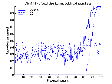
Figure 23 The performance for a system with a plastic projection between the LTM and STM. Different representation of the data was used in the LTM and STM.

4.3 Summary

A basic question was if two separate networks with different plasticity works better then one single network with two recurrent projections with different plasticity. It was concluded that a separation of neurons into two networks with different plasticity was good. It could also be established that two networks with different plasticity could be made to work together.

The concept with plastic projection between the LTM and STM was seen to work. It was also established that if a LTM and a STM were connected with plastic weights, the data could be represented differently in the two networks.

The constant g^STM^®LTM was introduced to provide an instrument that could control the level of influence between the networks of different plasticity. If g^STM^®LTM was set to 1, the STM had a dominant influence on the LTM. When g^STM^®LTM was set to 1 the LTM had problems to retrieve old patterns that were not stored in the STM.

5.0 Properties of connected networks

Chapter 4 was concerned with the disruptive influence of the STM on the LTM. A paradigm of the system design in chapter 4 was not to let the STM interfered the LTM capability to retrieve old memories. The goal of the experiments in chapter 5 was to provide an information base that could be used to design the systems of chapter 6, which incorporated a STM that functioned as a working memory.

5.1 Systems with reduced size of the STM.

The LTM stores all memories, although the most recent learned memories are not given precedence over older memories. The role of the STM is to give the latest learned memories such precedence. The STM can achieve this without having to store the latest memories. Remember that the STM in chapter 4 stored whole patterns. Instead of storing the patterns, the STM in 5.1 will hold pointers to the latest acquired memories. Each of these pointers in the STM will be pointing at a particular memory in the LTM. On retrieval of one of those particular memories the pointer will become active and aid the retrieval of the memory.

In cognitive psychology chunking is a popular concept. The compressed representation in the STM can be considered as a chunk representing the content in the LTM.

The experiments in 5.1 were designed to find out how a compressed STM could be constructed. Different representations in the STM were tried. An investigation of different sizes of the compressed STM was also performed. Note that when the system was in operating mode, the activity was first propagated from the LTM to STM. Then the activity was propagated back into the LTM. This was a big change from the systems in chapter 4, where the STM was directly fed with activity.

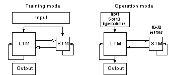
Figure 24 The design outline of the system in 5.1.1-5.1.3. Note that during operation the activity in the LTM is propagated through plastic projection to the STM, then the activity is propagated back to the LTM. The STM consisted of 10-30 neurons.

The systems in 5.1 were comprised of a LTM and a smaller STM. The LTM and STM were connected in both directions with plastic projections. Each of the systems was designed with three different sizes of the STM; 10, 20 and 30 neurons.

The plastic projections were trained with a_projection = 0.5. The constant g was set to 1 in both directions. The systems were trained with 50 patterns. This implied that that the LTM were able to learn all of the patterns.

The retrieval of the patterns was initiated by presenting the system with 5 hypercolumns of the patterns. The remaining 5 hypercolumns were left blank. (The activity for all units was set to zero.)

5.1.1 STM as a subset of the hypercolumns in LTM

Here, the STM was constructed through a sub-sampling of the hypercolumns in the LTM. The STM with 10 neurons was constructed simply through copying the content of the first hypercolumn in the LTM. The STM with 20 neurons was constructed out of the first two hypercolumns in the LTM. The STM with 30 neurons was constructed out of the first three hypercolumns in the LTM. This meant that just a few of the attributes (hypercolumns) of an object (memory) was accommodated by the STM. These few attributes were stored with the full depth of detail retained.

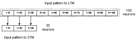
Figure 25 The outline for how the input patterns were constructed. The input to the 30 neurons of the STM was constructed out of the input to the first three hypercolumns of the LTM. When the STM is constructed with 10 or 20 neurons 1 or 2 hypercolumns of the LTM are used.

Figure 26 shows how the systems retrieval-ratio with three different sizes of the STM. The system with only 10 neurons in the STM (dash-dotted line) seemed to generate the best result.

A STM with only 10 neurons have less influence on the LTM then a system with 30 neurons has. The STM consisting of 10 neurons generate a projection on to the LTM containing 10x100 = 1000 elements, while a STM consisting of 30 neurons generate a projection with 30x100 = 3000 elements. A STM consisting of 30 neurons generates a more distinct retrieval suggestion to the LTM than a STM consisting of 10 neurons. Setting the constant g^STM^®LTM to a value less then 1 can adjust the influence of the STM.

It was interesting to see that even a small STM was able to help the LTM to activate the 10 latest patterns correctly. This effect confirms the idea that the STM doesn’t need to contain any information of the patterns, but instead can act as a pointer to the patterns stored in the LTM.

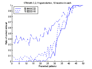
Figure 26 Three systems with different size of the STM are shown in the plot. Presenting the systems with 5 out of 10 hypercolumns tested the retrieval-ratios of the systems.

5.1.2 STM as a sub-sampled set of the hypercolumns in LTM

The LTM was in this experiment constructed through a compression of each hypercolumn in the LTM. The STM contained the same number of hypercolumns as the LTM (10). Each hypercolumn in the STM was comprised of 1, 2 or 3 neurons. This meant that all the attributes of an object was stored in the STM, but with less detail. This approach was the opposite of the approach taken in 5.1.1.

Note that the case where each of the hypercolumns in the LTM was represented by a single neuron in the STM was trivial. All of the neurons in the STM will always have the activity set to 1.

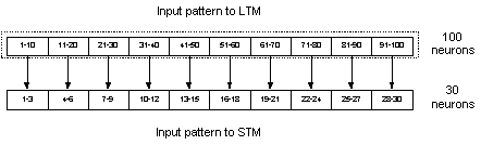
Figure 27 The outline for how the input patterns were constructed. Data within each hypercolumn was compressed. All of the 10 hypercolumns of the LTM are represented in the STM with 1, 2 or 3 neurons.

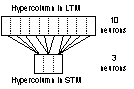
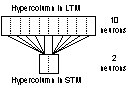
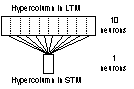
Figure 28 The figure shows how the hypercolumns in the LTM was transformed to the hypercolumns of the STM. The left figure corresponds to the case where the STM consisted of 30 neurons. The figure to the right corresponds to a system with a STM of 10 neurons. Note that the right figure is trivial.

The patterns stored in the STM were highly correlated since each hypercolumn only had 1, 2 or 3 different attribute values. Instinctively, this leads one to believe that the system should have a poor performance; especially when the STM is composed of 10 neurons. A STM composed of 10 neurons divided into 10 hypercolumns is not able to hold any information; all units would always be active. This was not the case, as can be seen in figure 29. The retrieval-ratio of this system and the system in section 5.1.1 was very similar. This can be explained with that much of the information is stored in the plastic projection between STM and LTM. The information stored in the STM seems to be of less importance.

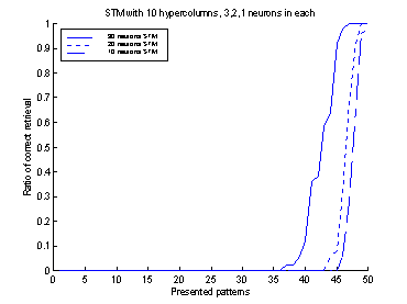
Figure 29 The performance for a system, where each hypercolumn of the LTM was compressed from 10 neurons to 3 neurons in the STM. Note that even the trivial case with 10 neurons, where all neurons are active in the STM, can hold information.

5.1.3 STM is a subset of sub-sampled hypercolumns

Anders Lansner [personal communication] have suggested that the relation between the number of hypercolumns and the number neurons in a network, for maximal capacity, should be

where H is the number of hypercolumns and N the number of neurons. In 5.1.3 the compression of the LTM was achieved through a compromise of sub-sampling and adopting a subset of the hypercolumns. The number of hypercolumns in the STM was chosen to follow the hypothesised relation.

The STM with 30 neurons had 6 hypercolumns. The STM with 20 neurons had 4 hypercolumns and the STM with 10 neurons had 2 hypercolumns. Each hypercolumn in the STM was consisted of 5 neurons.

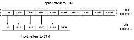
Figure 30 Shown here is the outline for how the input patterns were constructed when the STM was made of 30 neurons. When the STM was constructed with 20 neurons it had 4 hypercolumns, and when it was constructed from 10 neurons it had 2 hypercolumns.

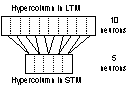
Figure 31 The hypercolumns of the LTM was compressed to half its size in the STM. This applied for all STM, independently of the number of neurons.

Figure 32 shows that the design approach provides good performance. The STM constructed in this manner holds more information then the STM of the two previous designs. It was interesting to see that the size of the STM did not affect the performance of the system.

Comparing the results of the experiments in 5.1, it is obvious that it is a good strategy to use a STM that has a sparse representation.

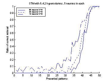
Figure 32 The performance for a system where the STM is a subset of sub-sampled hypercolumns of the LTM. Note that the size of the STM does not affect the performance of the system.

5.2 Interfering effects

When faced with the task of design there are often several parameters that can be adjusted in the system. Section 5.2 contains an investigation on how some of the most important parameters affect a system.

5.2.1 Effects of LTM on STM

In these two experiments, the focus was on how the plastic projection from the LTM to the STM affected the performance of the whole system. As in 5.1 the activity of the LTM was propagated to the STM and then back to the LTM. The phenomenon of interest in these two experiments was the self-induced interference generated by the LTM. In the two following experiments a plastic projection was used from the LTM to the STM. One of the experiments used a plastic projection with a high plasticity, and the other experiment used a plastic projection with low plasticity.

The STM and LTM were of equal size, 100 neurons. The STM had a set to 0.5. The system had a one-to-one projection from the STM to the LTM. The diagonal elements of the projection were set to the value 10. The choice of the value 10 caused some impairment of the LTM ability to recall old patterns.

From the LTM to the STM there was a plastic projection. In the case of low plasticity a_projection was set to 0.005 and in the case of high plasticity a_projection was set to 0.5. The plastic projection^LTM^®STM was scaled with g^LTM^®STM. Note that in this experiment, the g^LTM^®STM constant applied to the projection from the LTM to the STM.

The system was trained with 50 patterns. The system was presented with noisy patterns to test the retrieval-ratio.

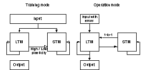
Figure 33 The system was used to test the effects of the connection strength from the LTM to the STM. The projection from the STM to the LTM was one-to-one and the diagonal elements were set to the value 10. From the LTM to the STM there was a plastic projection.

In figure 34 and figure 35 the retrieval-ratio for the two systems is seen. The value of g^LTM^®STM didn’t seem to affect the system as long as it was small. When the value of g^LTM^®STM exceeded exp (3) » 20 a steep fall in performance for both the systems was seen. Most likely this performance drop could be accredited to too much excitation of the STM. The projection^STM of the STM have up to this point, g^LTM^®STM = exp (3) » 20, been able to suppress the activity imposed by the LTM.

The system with high plasticity projection^LTM^®STM had a constant performance for the last 10 patterns, independently of the value of g^LTM^®STM. While the performance for the first 40 patterns slowly deteriorated as the value of g^LTM^®STM increased. When g^LTM^®STM exceeded 20 the performance of the system drastically dropped. The fact that the performance for the last 10 patterns remained constant was logic since we used a projection with high plasticity. As the influence of the LTM on the STM increased, the memories in the STM were reinforced.

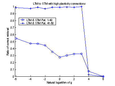
Figure 34 The system projection between the LTM and STM had high plasticity.

The system with low plasticity projections had a slowly deteriorating performance for the last 10 patterns as the value of g^LTM^®STM increased. The performance for the first 40 patterns was independent of the value of g^LTM^®STM. When g^LTM^®STM exceeded 20, the performance drastically dropped as in the other system. The fact that performance for the last 10 patterns slowly decreased, as the influence of the LTM on the STM increased (larger g^LTM^®STM), was logical since the system had low plasticity projection, which is not good at storing the most recently learned patterns.

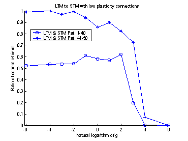
Figure 35 A system with a low plasticity projection between the LTM and STM.

5.2.2 Effects of STM on LTM

The projection in the direction from the STM to the LTM is more important than the reciprocal projection, since the state of the LTM is equal to the systems output. In this section I looked at the influence of the projection from the STM to LTM was studied. First a system with only one-to-one projection between the STM and LTM was studied. Then a system with a LTM and STM of equal size with plastic projection was studied. Finally a system with a compressed STM and plastic projection was studied.

The first system was constructed as the system in figure 15. The system had a fixed 1-to-1 projection from the STM to the LTM, with the value 10. When the system was operated, noisy input was fed directly to both the LTM and the STM. The LTM had a set to 0.005 and the STM had a set to 0.5. The systems were trained with 50 patterns.

Figure 36 shows the performance of the system with a 1-to-1 projection^STM^®LTM. When the value of the elements (weights) in the projection was smaller than exp (-2) » 0.1 a decrease in the performance of the most recently learned patterns was seen. This decrease seemed to be linear in respect to the logarithm of the weights. It was also interesting to see that the retrieval-ratio of the older patterns was not affected when the weights were smaller than 0.1.

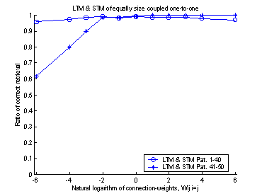
Figure 36 A system with a 1-to1 projection from the STM to the LTM. The system was tested with different values of the weights.

In a comparison between figure 36 and 37, it is seen that a 1-to-1 projection (figure 37) does not interfered the LTM as much as plastic projection does.

The second system was constructed with a STM and a LTM of equal size. The system design can be seen in figure 18. The projection^STM^®LTM from the STM to the LTM was plastic. The plastic projection was trained with a_projection set to 0.5. The system was trained with 50 patterns. The retrieval-ratio was tested with noisy patterns that were fed to both the LTM and the STM.

The performance of the second system is shown in figure 37. The retrieval-ratio, for the last 10 patterns, fall sharply when the value of g^STM^®LTM exceeds exp (3) » 20. The retrieval-ratio for the first 40 patterns starts to fall when the value of g^STM^®LTM exceeds exp (-3) » 0.05.

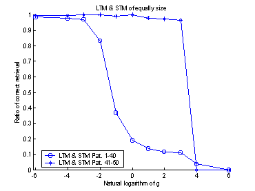
Figure 37 A system with equal size of the LTM and STM. The plastic projection was trained with a set to the value 0.5.

The last experiment was made with a system similar to the one in figure 18. The difference was that this system had a reduced size of the STM. When operated, the system was fed with input directly to both the LTM and STM. The input to the LTM had errors, while the input to the STM had no errors. The STM was made of 30 neurons. The input to the STM was the same as the input to the first three hypercolumns of the LTM.

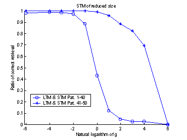
Figure 38 In this experiment the system has a smaller STM then in the previous experiment.

The retrieval-ratio of the first 40 patterns is similar to that of the previous experiment. The retrieval-ratio of the last 10 patterns starts to drop earlier than in the previous experiment. The gentler drop of the retrieval-ratio of the last 10 patterns seen in this experiment compared with the previous experiment can be accredited to the reduced influence of the compressed STM.

5.3 LTM helped by STM on retrieval

How much information is needed to retrieve a pattern in LTM and how does a STM affect the retrieval? These two questions were answered by the experiment in 5.3. These two questions become very relevant when one design a system where the patterns are dived into individual modules, as in chapter 6.

The same system as in 5.1.1 was used. The STM was composed of 30 neurons divided into 3 hypercolumns. The first three hypercolumns of the patterns were stored in the STM. The system is shown in figure 24. The system was run with four different values of g^STM^®LTM. The g^STM^®LTM scaled the projection from the STM to the LTM. The pattern retrieval was initiated with 1 to 5 of the hypercolumns constituting the learned patterns.

In figure 39A one can clearly se how the STM interfere the LTM. The STM have a positive effect on the retrieval of the most recent patterns. Even though only the information of one hypercolumn is presented to the system, it can retrieve the correct pattern.

In figure 39D the retrieval-ratio of a system that does not have any STM is seen. If the system is only presented with one hypercolumn, the retrieval-ratio becomes very low. The system needs to be presented with 4 hypercolumns before the retrieval-ratio becomes good.

A B

C D

Figure 39 Illustration of how the STM affects retrieval of memories in LTM. Upper left plot have g^STM^®^LTM =1, upper right g^STM^®^LTM =0.5, lower left g^STM^®^LTM =0.1. In the lower right plot, the system has no STM.

5.4 STM ability to suppress old information in the LTM

This experiment was designed to verify that a system composed of a LTM and STM put most significance on the latest learned patterns. This means that if two patterns are very similar, and the system is asked to retrieve one of these patterns it should retrieve the most recently learned pattern. This also connects to the concept of STVB.

The system used was identical to the system in 5.1.1 with a STM composed of 30 neurons. The patterns used as input to the system consisted of two parts, called “Tag” and “Content”. The input to the STM was the part of the pattern called “Tag”. The “Tag” can be seen to represent a variable while the “Content” is representing the content of the variable.

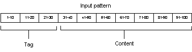
Figure 40 A pattern, with the parts tag and content defined. The tag is represented by the first 3 hypercolumns, and the content is represented by hypercolumns 4 to 10.

The system was trained with 50 patterns. The first pattern presented to the system, pattern A, was repeated a number of times. The 48:th pattern was called pattern B. Patterns A and B were very similar, their first six hypercolumns were identical.

When all of the 50 patterns had been presented and learnt by the system, the first six hypercolumns of pattern A (the first six hypercolumns of patterns A and B were identical) was presented to the system. The system now had the choice of converging to pattern A or B. The result is shown in figure 41. The system was run without the STM and the result of this run is shown in figure 42. It may look strange that the retrieval-ratio is sometimes larger than 1. The cause to this odd characteristic is that sometimes the last 4 hypercolumns of the patterns A and B are similar enough to cause both patterns, A and B, to be collapsed into one single pattern.

The system in this experiment performs a STVB task. The example of STVB given in 2.5.1, described how John knew if he was talking to his grandfather, named Sven, or his friend, also named Sven. To manage this task, John had to know which of these Sven’s he most recently had met. The system in this experiment is presented with a similar task. To refer to the example given in 2.5.1; the name of a person is in this experiment is represented by the “Tag” and a physical person is represented by the “Content”. Pattern A can be seen to represent John’s grandfather, named Sven, and pattern B to represent John’s friend, also named Sven. The repeated training of pattern A (representing the grandfather) can be seen as a long conversation with the grandfather. The problem the system now face, is that even if the systems has had a long talk to the grandfather, as soon as the system starts to talk to the friend, the system knows directly that it is not talking to the grandfather any more. To manage this task, the system needs to swiftly change its references. The STM plays a crucial role in the swift change of references.

In the first experiment where the STM was enabled, the system almost only retrieved the latest learned pattern, pattern B. (Figure 41)

Figure 41 This histogram shows that the system’s retrieval-ratio of the latest learned pattern, B. The retrieval-ratio of pattern B was tested after different amounts of training with pattern A. Pattern A and B had the same “Tag”. The figure shows, that if pattern A had been trained 20 times, the system retrieved the most recent pattern, pattern B.

When the system’s STM was disabled (Figure 42), the system only retrieved pattern B as long as the pattern A had not been trained extensively. Once pattern A had been trained 3-4 times, the system almost never retrieved pattern B.

Figure 42 The performance the system, when the STM was disabled. When pattern A has been repeated more than 2 times it is almost impossible for the system to retrieve pattern B.

This experiment shows that a STM can have a great impact on the system’s behaviour. White the STM, the system could easily change the binding from the name variable to a new content. Without the use of a STM, the system could not perform this task well.

5.5 Summary

The fundamental concept that the STM does not need to contain the whole patterns that are stored in the LTM was tried. 3 different approaches were taken to the design of the STM. It was seen that the approaches that generated a sparse representation in the STM was generally good. It was concluded that the STM only needed to be able to store as many distinctive memory traces as the memory were supposed to hold. In our case this meant that the STM should be able to hold about 10 distinct memory traces. The information of particular patterns was stored in the projection between the STM and LTM.

An investigation of how the LTM and STM interfered each other was preformed. It was concluded that that the interfering effect off the LTM on the STM was minimal. But if g^STM^®LTM was made bigger than 20 a drastic drop in the retrieval-ratio occurred.

It was also studied how the STM interfered the LTM. If the two networks were connected with a 1-to-1 projection, the interference was minimal. The disruptive effect became much larger when plastic weights were used. It was established that a smaller STM interfered the LTM less then a large STM.

An experiment was performed to investigate how much data a system of LTM and STM needed to retrieve a memory (pattern). We concluded that a recent memory could be retrieved after presenting the system with two hypercolumns. To retrieve an older memory the system needed to be presented with information of four hypercolumns.

Finally we saw that a memory system with both a LTM and STM, always gave precedence to the most recently learned memories.

6.0 STM used as working memory

Chapter 6 studied how a STM can be implemented as a working memory. Two different systems were studied. The system in 6.1 was based on a single STM and a single LTM. The system in 6.2 was constructed with modules that were built of one LTM and one STM. These two systems were tested on the task presented in figure 42.

There are 4 different places, Place 1-4. In each place a box can be placed. There are 4 different boxes, Box 1-4. Each box has a certain content. If there are 4 boxes, there are 4 different contents, Content 1-4, one for each box. The task was to keep track of the boxes as they moved around to different places. The working memory is supposed to hold the information that Box 1 and Box 2 have switched place. The long-term memory holds the information about what content each box has. It means that the systems need both a long-term memory and a working memory to be able to perform the task.

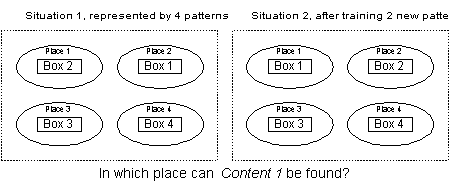
Figure 43 The system is first presented with Situation 1, then Situation 2. After this two situation has been presented, the system is asked to retrieve the place where “Content 1” is stored. The 4 places are supposed to be well known. The 4 different boxes and their individual content are also supposed to be well known. This task is presented to the two systems in 6.1 and 6.2.

6.1 System based on LTM and STM

The purpose of this experiment was to show that a STM could function as a working memory. The system was built with one LTM and one STM. In section 6.2, a modified version of this system was used as a module in a larger system.

The system used was almost identical to the system in 5.1.1 with 30 neurons in the STM. There were two differences. The first difference was that the input to the STM was taken from hypercolumns 4-6 of the patterns. (Instead of the first 3 hypercolumns. This difference is totally negligible.) The second difference was that only the first 6 hypercolumns of the LTM were connected to the STM.

The patterns were composed of three different parts as seen in figure 44. There were 4 different places. There also were 4 different boxes. Each box had a particular content specific to that particular box.

Figure 44 The input to the system had the structure outlined here. Each Box had a certain Content. Each box was placed in a certain Place. There were 4 places and 4 boxes with their individual content.

The system was trained 2 times with all possible combinations of boxes, and their content, in different places (16 different combinations). The purpose of this training was to learn the system each of the four “box-content” constellations. After these 2*16=32 patterns had been presented to the system, the system was presented with 10 patterns that contained noise. The last six patterns were more intricate. Pattern 43-46 corresponds to situation 1 in figure 43. Pattern 47-48 corresponds to situation 2 (only the novelties in the new situation were learned) in figure 43. All patterns, 1-48, are documented in table 1.

Pattern No	Place	Box	Content
1-16	X	Y	Y
17-32	X	Y	Y
33-42	Noise	Noise	Noise
43	1	2	2
44	2	1	1
45	3	3	3
46	4	4	4
47	1	1	1
48	2	2	2

Table 1 This table shows the training set of 48 patterns. Pattern 1-16 contain all possible combinations of X and Y where X, Y Î {1,2,3,4}.

When the system was tested, it was presented with the four different contents, Content 1-4. The system was then asked to retrieve the corresponding “Box” and “Place” to each “Content”.

The system’s LTM associated each “Content” to its corresponding “Box”. The “Box” in turn associated itself to the correct “Place” using the working memory.

In table 2 the result of the run is shown. Naturally, the retrieval-ratio of the content is 1. The retrieval-ratios for the Box and the Place are also almost 1. Note that the system has no problem too keep track of the last minute switch of Place between Box 1 and Box 2.

Fraction of correct retrieval of:	Content	Box	Place
Box 1	1.00	0.98	0.98
Box 2	1.00	0.99	0.92
Box 3	1.00	1.00	0.99
Box 4	1.00	1.00	1.00

Table 2 The performance of the system. The system was fed with a “content”, and then asked to retrieve the place where this content was.

The same system was tested with the STM disabled. The result is shown in table 3. The retrieval-ratio of the content and box was still 1. This is what could be expected since the retrieval of the “Box” is made with the LTM. It was interesting to see what happened to retrieval of the “Place”.

The “Place” where Box 3 and Box 4 were put, was retrieved approximately 25% of the times. This corresponds to the random frequency, when picking between four equal likely alternatives. The same retrieval-ratio, 25%, of the “Place” were Box 1 and Box 2 were placed, was expected. Instead I found the retrieval-ratio to be zero in these two cases. This was strange.

Probably, the reason to the zero retrieval-ratio was that the convergence was slower. All of the system in this thesis used a fixed convergence-time of 1 time-unit. The convergence-time in this case was probably up to 10 time-units. I did not depend the investigation into this matter, since I did find relevant to the working memory.

Fraction of correct retrieval of:	Content	Box	Place
Box 1	1.00	1.00	0.00
Box 2	1.00	1.00	0.00
Box 3	1.00	1.00	0.26
Box 4	1.00	1.00	0.32

Table 3 The result of the system with the STM disabled. Note that the system can not keep track of the switch between box 1 and 2.

6.2 System built with modules of LTM and STM

The aim of this experiment was to show that a modular system could be designed and that this modular system could perform equally well as the “integrated” system in 6.1. In this new modular system, the representation of the Box/Content and the Place was separated into separate modules. The approach, of constructing the systems with LTM & STM modules, has many benefits over the systems with a single LTM & STM. If the system is required to handle a new type of input / class of attributes, it is easy just to add a module. And if the properties of a certain class of attributes are altered, it is easy to alter the corresponding module.

The modular system is based on two modules, each module contain a LTM and a STM. This system was tested on the same task as the system in 6.1. Each of these modules is identical to the system in 5.1.1. The STM contain 30 neurons and is connected to the LTM with a plastic projection. Figure 45 shows the modular system. The bi-directional projection between STM 1 and STM 2 has a_projection set to 0.5. The projections from STM 1 to LTM 2 and STM 2 to LTM 1 also have a_projection set to 0.5. The bi-directional projection between LTM 1 and LTM 2 had a_projection set to 0.005. The projections between LTM 1 and LTM 2 were made spares by random deletion of 70% of the elements in the projections. The deletion of these elements made the separation between the modules more clear. The aim was to minimize the number of connection between the modules.

Figure 45 A system constructed of two smaller systems from section 5.1.1. This system shows how bigger systems can be constructed out of smaller modules. The system has two LTM connected with sparse plastic projections, and two STM connected with plastic projections.

In 6.1, all information was stored in the single LTM. In this system, the “Place” and “Box / Content” memories are stored in two separate LTM. Figure 46 shows how the “Place” memories are represented in LTM 1. Figure 47 shows how the “Box / Content” memories are represented in LTM 2. If the system is equipped with a third module, the representation of the “Box / Content” can be separated.

Figure 46 The input to module 1 of the system.

Figure 47 The input to module 2 of the system.

The system was trained with the set of patterns described in table 1. The system was trained on each pattern during 1 time-unit. On retrieval the system was fed with each of the four ”Content”. Retrieval (relaxation) was also made during 1 time-unit. The output was taken from both LTM 2 and LTM 1.

The retrieval process of the “Place” memory started with input of the “Content”. The system then used the LTM 2 to activate the “Box” memory. The “Box” memory then activated the “Place” memory, using the STM projections on LTM1.

The performance of the system was good. Table 4 shows the result of 100 runs. This result shows that the modular design is working well.

Fraction of correct retrieval of:	Content	Box	Place
Content 1	1.00	1.00	0.99
Content 2	1.00	1.00	0.97
Content 3	1.00	1.00	0.99
Content 4	1.00	1.00	1.00

Table 4 The performance of the modular system, when executing the task described in the beginning of chapter 6.

Table 5 shows the result of a run with the system where the two short-term memories, STM 1 and STM 2, have been disabled. The retrieval-ratio of the “Place” memories is very poor. This is expected, since the retrieval of these memories is dependent on the working memory. If the result in table 5 is compared with the result in table 3, one finds that the retrieval-ratio for “Content 1” and “Content 2” is no longer zero, and the retrieval-ratio for “Content 3” and “Content 4” has increased. As I earlier stated, these differences can be traced back to the relaxation time and the different networks structures and data representations.

Fraction of correct retrieval of:	Content	Box	Place
Content 1	1.00	1.00	0.14
Content 2	1.00	1.00	0.23
Content 3	1.00	1.00	0.40
Content 4	1.00	1.00	0.37

Table 5 The performance of the modular system, when the STM 1 and STM 2 were disabled.

This experiment shows that several Bayesian networks can be used in a modular designed system. The experiment also, once again, proved the usefulness of a working memory. It remains to be studied how these modular system scales.

6.3 Summary

It was shown that a STM, based on a attractor network, could function as a working memory. We could also see that a system with both a LTM and a STM could solve problems that would not have been possible to solve with a system comprising of only a LTM or a STM.

Larger systems, based on modules of LTM and STM, was constructed. We concluded that these systems could be applied to solve the same problem as the smaller system, based on a single LTM and STM. The advantages of the modular system were that its capabilities easily could be extended and modified.

1.0 Introduction